

This is not a trick: the cosine of the imaginary number 𝑖 is (e⁻¹ + e)/2.
How on Earth does this follow from the definition of the cosine? No matter how hard you try, you cannot construct a right triangle with an angle 𝑖. What kind of sorcery is this?
Read on to find out.
How on Earth does this follow from the definition of the cosine? No matter how hard you try, you cannot construct a right triangle with an angle 𝑖. What kind of sorcery is this?
Read on to find out.

First, the fundamentals.
In their original form, trigonometric functions are defined in terms of right triangles.
For an acute angle α, the sine and cosine are given by the ratio of the appropriate leg and the hypotenuse. (This is visualized below.)
In their original form, trigonometric functions are defined in terms of right triangles.
For an acute angle α, the sine and cosine are given by the ratio of the appropriate leg and the hypotenuse. (This is visualized below.)

Is this a proper definition? Doesn't it depend on the choice of the triangle?
Even though the sine and cosine formally depend on the sides, they remain invariant to translating, scaling, rotating, and reflecting the triangle.
Even though the sine and cosine formally depend on the sides, they remain invariant to translating, scaling, rotating, and reflecting the triangle.

In other words, the trigonometric functions are invariant to similarity transformations. Thus, sine and cosine are well-defined: they depend only on the angle α.
Because of this, basic trigonometry is used to measure distances. Imagine a lighthouse towering in the distance. If we know its height and measure its angular distance, we can calculate how far the top of the tower is from us using sine and the Pythagorean theorem.
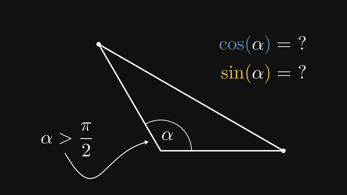
What about angles larger than π/2 radians? (Or 90°. But radians are infinitely cooler.) In this case, there is no right triangle, no hypotenuse, and no legs either.
We can find the answer by giving a clever representation of the trigonometric functions.
We can find the answer by giving a clever representation of the trigonometric functions.
If we move over to the Cartesian coordinate system, we can form a right triangle such that
• its hypotenuse is a unit vector,
• and its legs are parallel to the 𝑥 and 𝑦 axes respectively.
Take a look at the illustration below.
• its hypotenuse is a unit vector,
• and its legs are parallel to the 𝑥 and 𝑦 axes respectively.
Take a look at the illustration below.
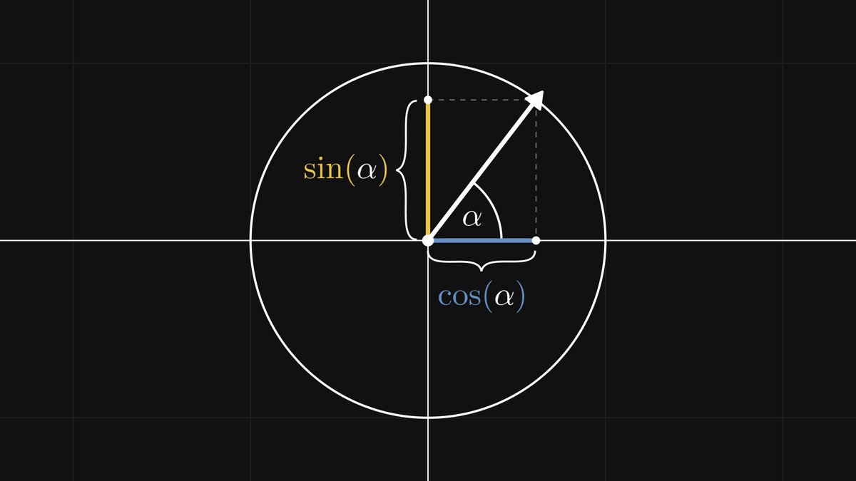
This way, the cosine and sine coincide with the 𝑥 and 𝑦 coordinates of our unit vector serving as the hypotenuse. Why is this good for us?
Because we can talk about obtuse and reflex angles! (That is, angles larger than π/2 radians.)
Because we can talk about obtuse and reflex angles! (That is, angles larger than π/2 radians.)
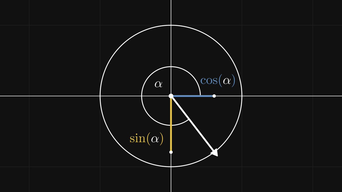
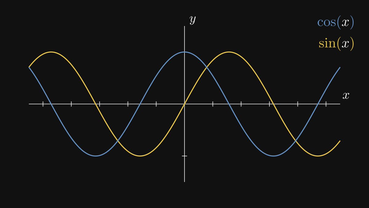
Finally, the definition for an arbitrary real α is complete if we consider that by winding the unit vector around, we can extend the trigonometric functions by periodicity.
(This works for both the clockwise and counter-clockwise directions.)
(This works for both the clockwise and counter-clockwise directions.)
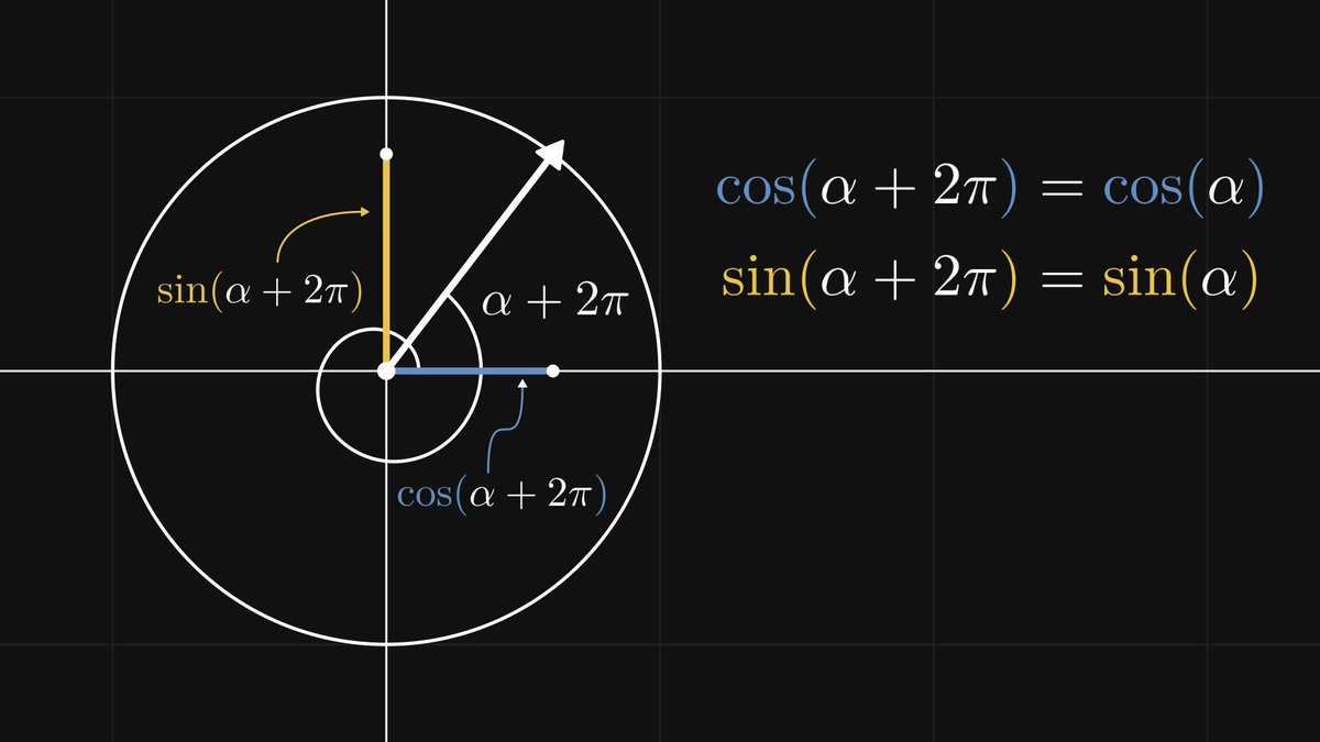
Thus, we get the familiar wave-like graphs. Here are sine and cosine, in their (partially) complete glory.
It’s great that we have defined sine and cosine for arbitrary real numbers, but there is one glaring issue: how can we calculate its value in practice?
For certain values, like π/4, we can explicitly construct a corresponding right angle and calculate the ratios by hand.
For certain values, like π/4, we can explicitly construct a corresponding right angle and calculate the ratios by hand.
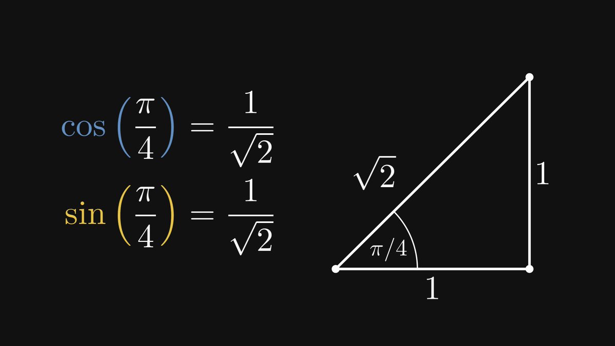
However, we can’t do this for any α. What to do then? Enter the Taylor polynomials.
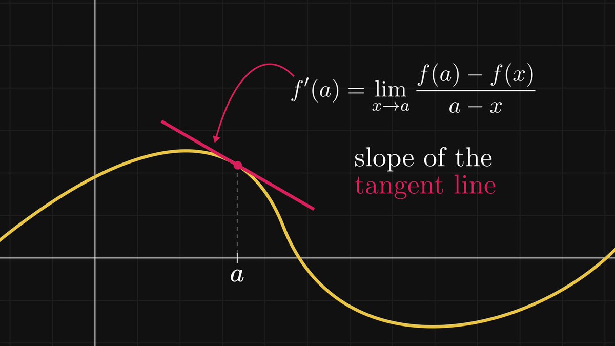
Let’s go back to square one: differentiation. By definition, the derivative of a real function describes the slope of the tangent line at the given point.
Let’s go back to square one: differentiation. By definition, the derivative of a real function describes the slope of the tangent line at the given point.
By knowing the derivative, we can write the equation for the tangent line.
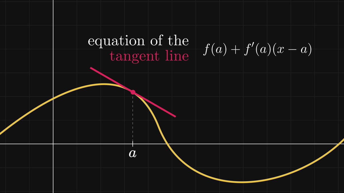
Again, why is this good? Because locally we can replace our function with a linear one, and linear functions are easy to compute!
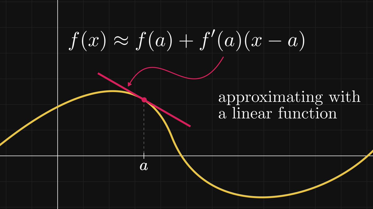
In fact, this is the best possible linear approximation. Can we do a better job with higher-degree polynomials?
Yes! It turns out that with the first n-th order derivatives, we can explicitly construct the best approximating polynomial of 𝑛-th degree.
Yes! It turns out that with the first n-th order derivatives, we can explicitly construct the best approximating polynomial of 𝑛-th degree.
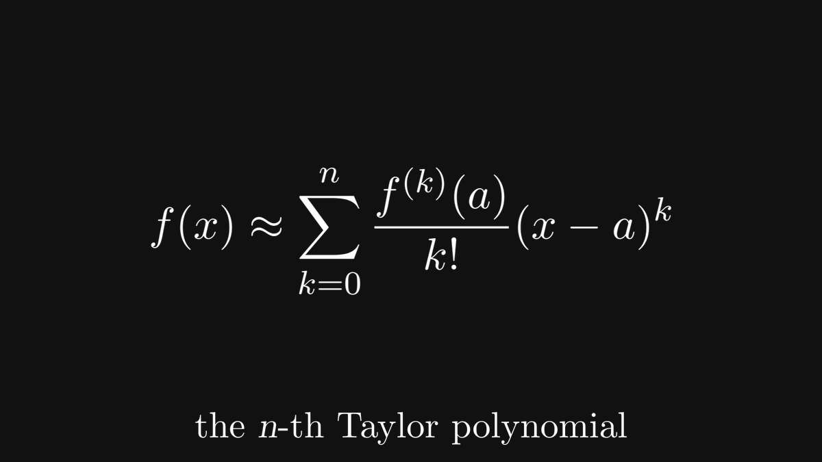
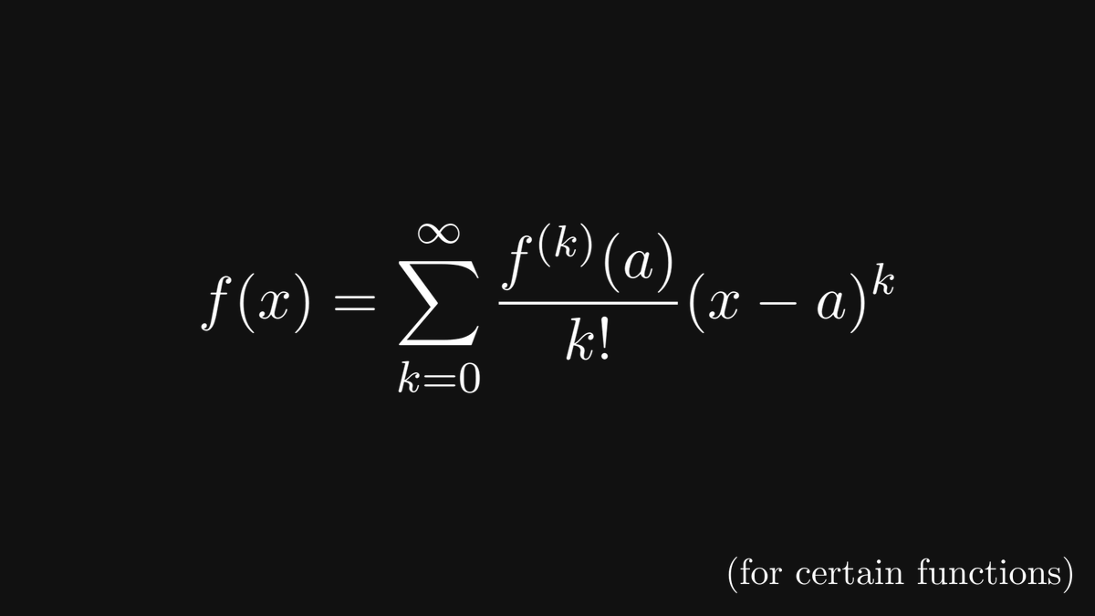
It gets even better: certain infinitely differentiable functions are exactly reproduced by letting the degree to infinity.
This is called the Taylor series around 𝑎. (Also called a power series.) The question: does this help us calculate the sine and cosine?
Yes, big time.
This is called the Taylor series around 𝑎. (Also called a power series.) The question: does this help us calculate the sine and cosine?
Yes, big time.
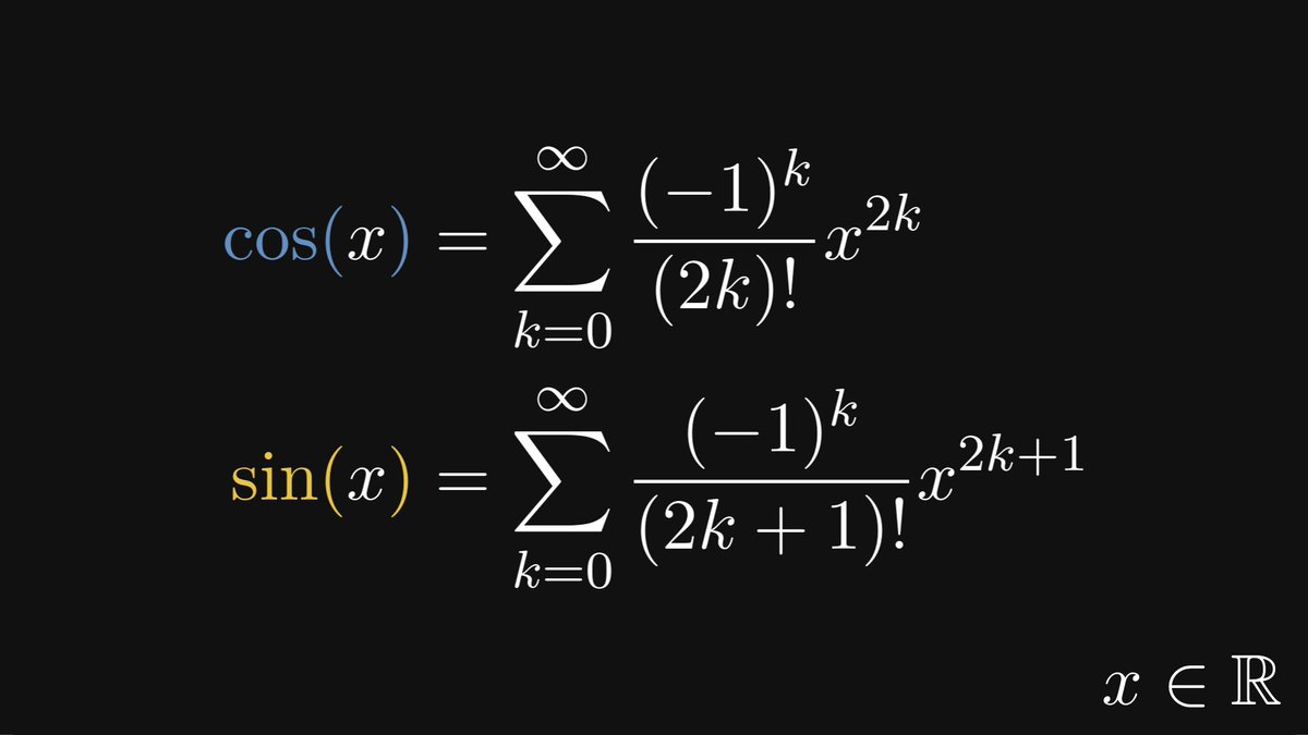
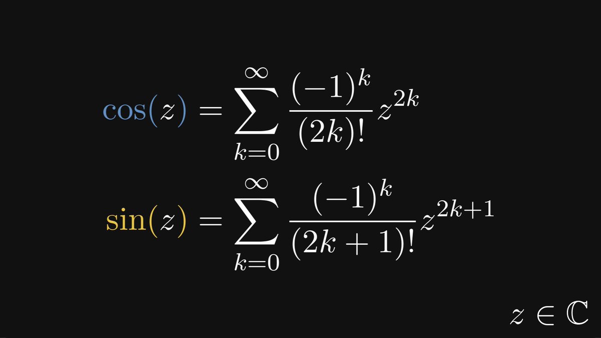
I’ll unveil the mystery without further ado: sine and cosine are reconstructed by their Taylor series around 0.
As sine and cosine are the derivatives of each other (up to a factor of -1), the Taylor series can be easily given.
As sine and cosine are the derivatives of each other (up to a factor of -1), the Taylor series can be easily given.
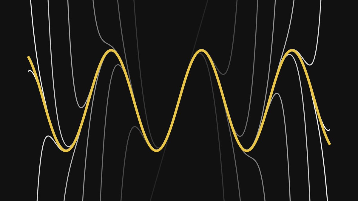
In practice, we compute finitely many terms, replacing the function with a polynomial. The higher the cutoff point, the better the approximation.
By plotting its Taylor polynomials along with the sine function, we see how the approximations eventually smooth over the function.
By plotting its Taylor polynomials along with the sine function, we see how the approximations eventually smooth over the function.
Now that we have a Taylor series representation, can’t we just plug in a complex number? After all, we can raise any complex number to any integer power, so nothing stands in our way.
And thus, extending the trigonometric functions to the complex plane comes for free.
And thus, extending the trigonometric functions to the complex plane comes for free.
Sounds simple enough. Is it useful? Yes. Let me show you the single most mind-blowing connection in mathematics: expressing the exponential function in terms of sine and cosine.
The Taylor series is like a Swiss army knife in mathematics. It’s not just for the sine and cosine; a lot of the important functions have a convergent Taylor series representation.
One such function is the famous exponential function, given by its power series below.
One such function is the famous exponential function, given by its power series below.

Besides the already discussed computational advantages, there is another one. And quite a surprising one to say the least!
By plugging in 𝑖𝑧 to the power series of the exponential function, a brief but tedious calculation gives us an unbelievable result:
By plugging in 𝑖𝑧 to the power series of the exponential function, a brief but tedious calculation gives us an unbelievable result:
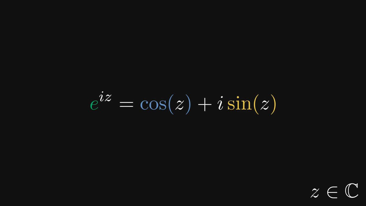
This is the famous Euler’s formula, connecting the complex exponential to trigonometric functions. (The original Euler’s formula is restricted to real numbers, but we’ll let this slide.)
With a bit of algebra, we can express sin and cos in terms of the exponential.
With a bit of algebra, we can express sin and cos in terms of the exponential.

Again, by plugging in 𝑧 = 𝑖 here, we show what was hinted at the beginning: the cosine of the imaginary unit 𝑖 is (e⁻¹ + e)/2.

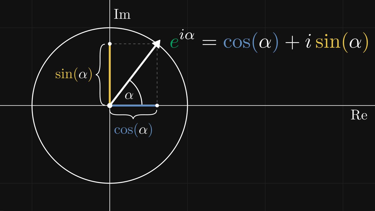
Euler’s formula is behind the polar representation of complex numbers as well. Previously, we have seen that the vector (cos(t), sin(t)) parametrizes the unit circle. Thus, by restricting Euler’s formula to the real numbers, we obtain the unit circle.
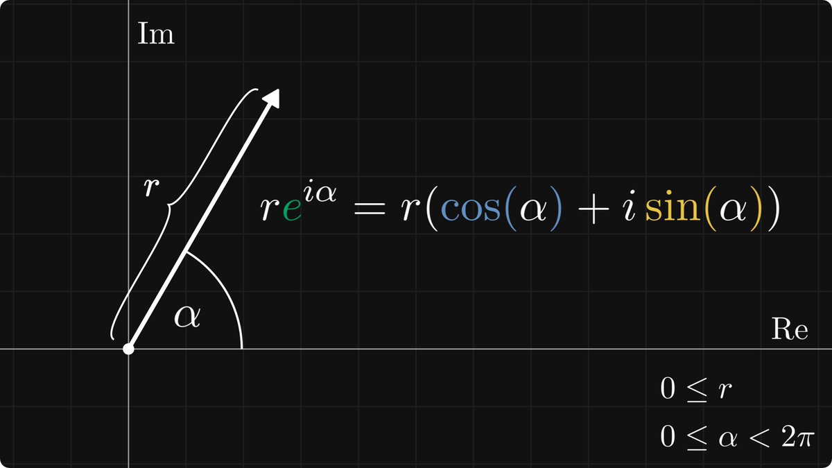
Any complex number can be described by its absolute value and its phase. (This is an alternative to the default representation provided by the real and imaginary units.)
Combining this with Euler’s formula, we obtain the so-called polar representation of complex numbers.
Combining this with Euler’s formula, we obtain the so-called polar representation of complex numbers.
Why is this useful? Check out how two complex numbers are multiplied.
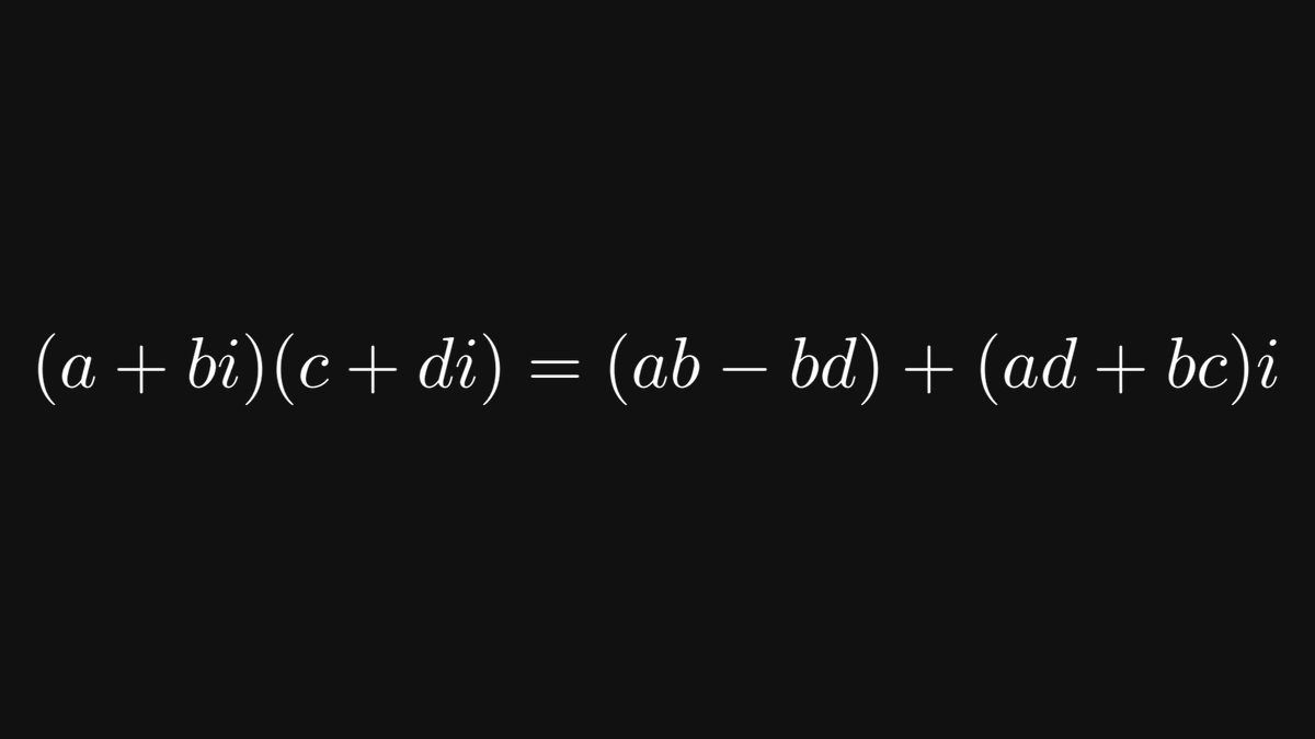
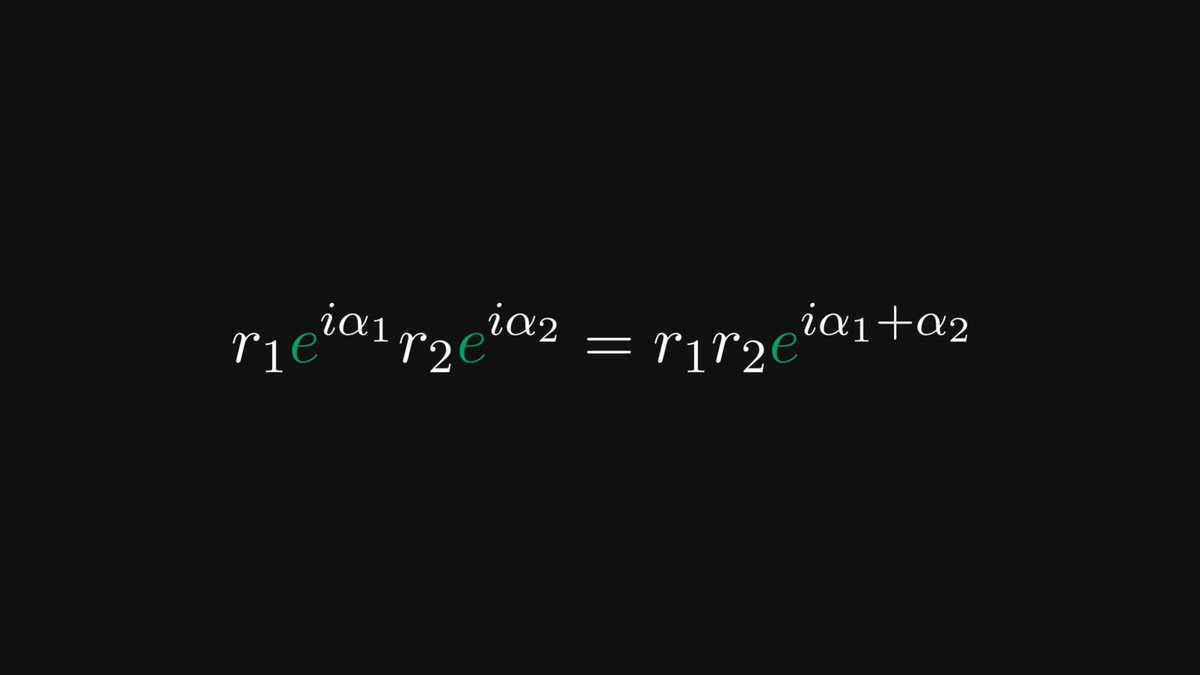
Now, the same with the polar representation.
The latter one is much more revealing. First, it is much simpler, but there is more. Polar representations provide a clear geometric picture: multiplication is stretching and rotation!
That’s a long way from right triangles.
The latter one is much more revealing. First, it is much simpler, but there is more. Polar representations provide a clear geometric picture: multiplication is stretching and rotation!
That’s a long way from right triangles.
Read the full version of the post here:
thepalindrome.substack.com
thepalindrome.substack.com
If you have enjoyed this thread, support me with a paid subscription to my newsletter!
(Or simply share this with your friends.)
Mathematics is neither dull nor dry; it’s beautiful, mesmerizing, and useful. Your support helps me show this to everyone.
thepalindrome.substack.com
(Or simply share this with your friends.)
Mathematics is neither dull nor dry; it’s beautiful, mesmerizing, and useful. Your support helps me show this to everyone.
thepalindrome.substack.com
Loading suggestions...