

Over 750 million people use Excel worldwide, yet 99% of them do not know how to use it effectively.
Here are the basic formulas that you should learn:
Here are the basic formulas that you should learn:
1. XLOOKUP
Use this function to search both vertically (by row) and horizontally (by column) in a table.
This is an upgrade compared to VLOOKUP or INDEXMATCH.
I'm looking for the revenue of a given product for multiple years.
The formula is =XLOOKUP(A11,A2:A8,B2:G8).
Use this function to search both vertically (by row) and horizontally (by column) in a table.
This is an upgrade compared to VLOOKUP or INDEXMATCH.
I'm looking for the revenue of a given product for multiple years.
The formula is =XLOOKUP(A11,A2:A8,B2:G8).

2. Pivot Tables
A pivot table is a powerful tool to calculate, summarize, and analyze data that lets you see comparisons, patterns, and trends in your data.
A pivot table is a powerful tool to calculate, summarize, and analyze data that lets you see comparisons, patterns, and trends in your data.

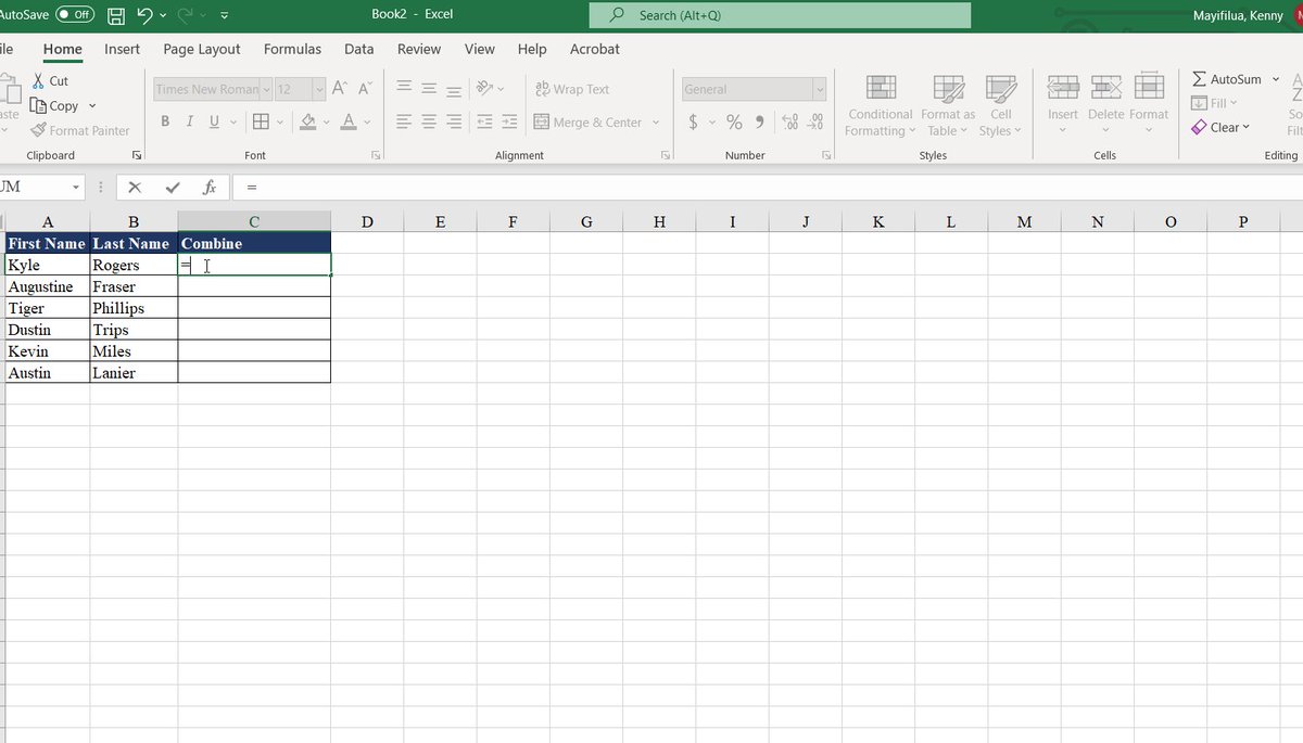
3. CONCATENATE
Use this function to join two or more text strings into one string.
I want to merge the first and last names into a single cell.
Don't forget the “ ” and the space in the middle if it's to separate the two texts.
The formula is =CONCATENATE (A2,“ ”,B2).
Use this function to join two or more text strings into one string.
I want to merge the first and last names into a single cell.
Don't forget the “ ” and the space in the middle if it's to separate the two texts.
The formula is =CONCATENATE (A2,“ ”,B2).
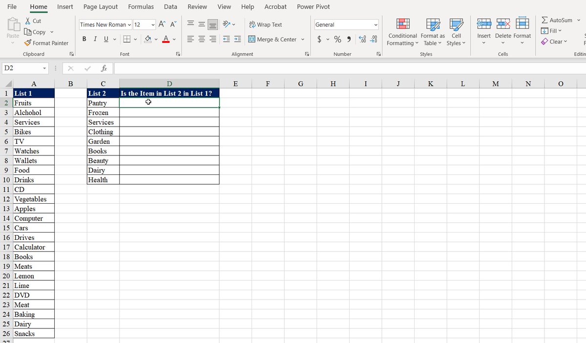
4. MATCH & ISNUMBER
MATCH searches and returns the position items in the range.
ISNUMBER checks whether a value is a number and returns True or False.
Only services, books, and dairy returned numbers are on both lists.
The formula is = ISNUMBER(MATCH(C2,$A2$:$A$26,0)).
MATCH searches and returns the position items in the range.
ISNUMBER checks whether a value is a number and returns True or False.
Only services, books, and dairy returned numbers are on both lists.
The formula is = ISNUMBER(MATCH(C2,$A2$:$A$26,0)).
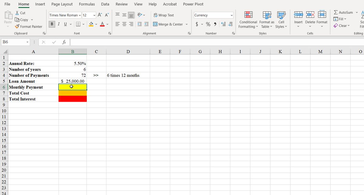
5. PMT
It calculates the payment for a loan based on constant payments and a constant interest rate.
This can be used to calculate a car loan or mortgage payment.
Put a negative in the function so that the result is positive.
The formula is = PMT(rate, nper, pv, [fv], [type])
It calculates the payment for a loan based on constant payments and a constant interest rate.
This can be used to calculate a car loan or mortgage payment.
Put a negative in the function so that the result is positive.
The formula is = PMT(rate, nper, pv, [fv], [type])
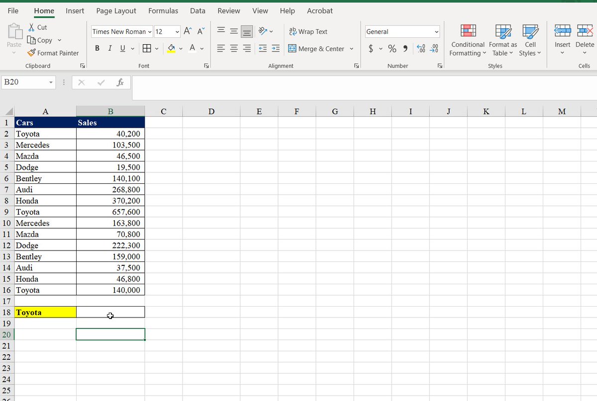
6. SUMIF
Use the SUMIF function to sum the values in a range that meets the criteria that you specify.
In this situation, I'm attempting to calculate the number of sales for a certain vehicle.
The formula is =SUMIF(A2:A16,A18,B2:B16).
Use the SUMIF function to sum the values in a range that meets the criteria that you specify.
In this situation, I'm attempting to calculate the number of sales for a certain vehicle.
The formula is =SUMIF(A2:A16,A18,B2:B16).
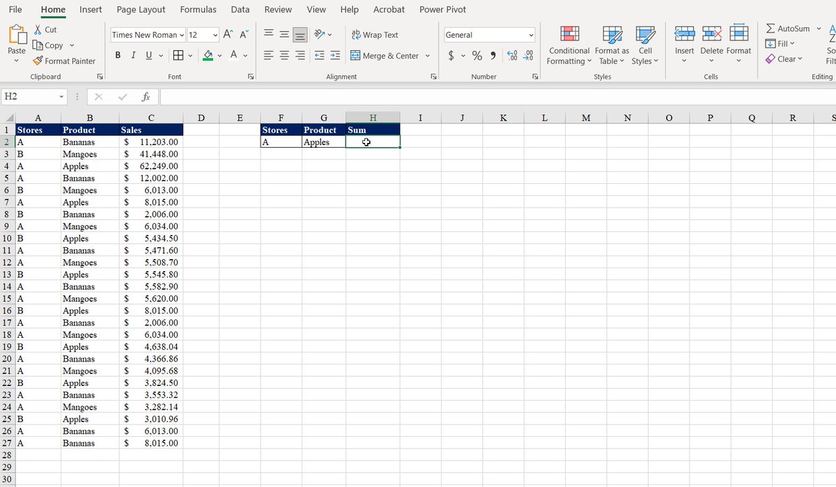
7. SUMIFS
SUMIFS is used to sum the values in a range that meets multiple criteria that you specify.
In the example, we want the sum of our two criteria, which are stores and products.
SUMIFS(sum_range, criteria_range1, criteria1, [criteria_range2, criteria2], ...)
SUMIFS is used to sum the values in a range that meets multiple criteria that you specify.
In the example, we want the sum of our two criteria, which are stores and products.
SUMIFS(sum_range, criteria_range1, criteria1, [criteria_range2, criteria2], ...)
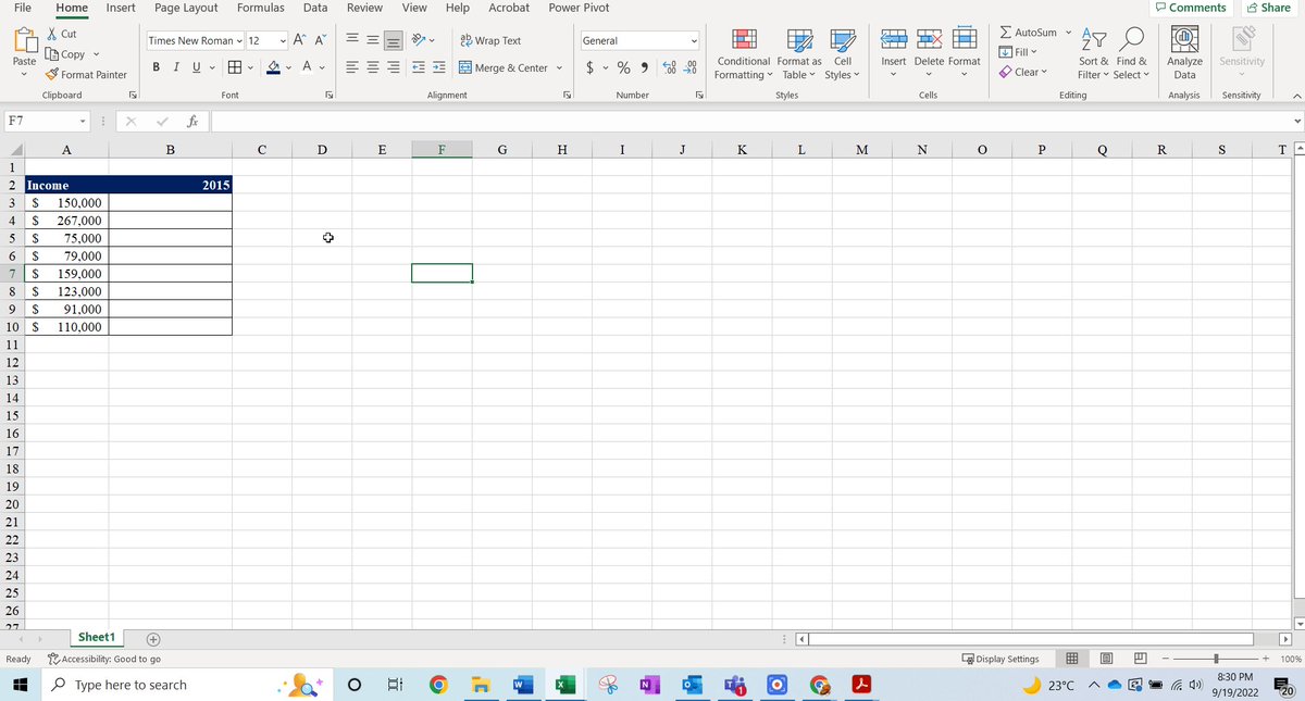
8.IF
Use the IF function to make logical comparisons.
The logical comparison is to use the word "rich" for revenue over $100,000.
If revenue is less than $100,000, it will return the word "Middle class".
The formula is =IF(A3>100000,"Rich","Middle Class").
Use the IF function to make logical comparisons.
The logical comparison is to use the word "rich" for revenue over $100,000.
If revenue is less than $100,000, it will return the word "Middle class".
The formula is =IF(A3>100000,"Rich","Middle Class").
9. COUNTIF
Use COUNTIF to count the number of cells that meet a criterion.
I'm keeping track of how many times these businesses have been the best in multiple years.
The formula is =COUNTIF(A2:B20,A23).
Use COUNTIF to count the number of cells that meet a criterion.
I'm keeping track of how many times these businesses have been the best in multiple years.
The formula is =COUNTIF(A2:B20,A23).

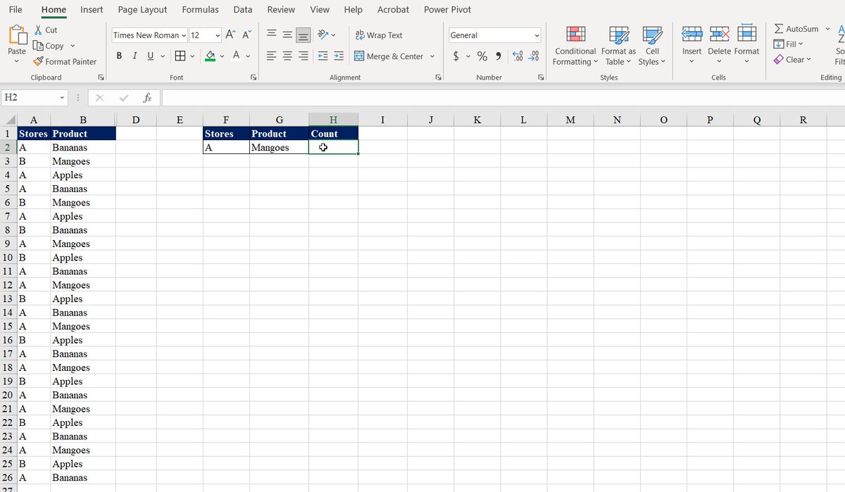
10. COUNTIFS
It applies criteria to cells across multiple ranges and counts the number of times all criteria are met.
Here, it counts the number of occurrences of a given store and product.
COUNTIFS(criteria_range1, criteria1, [criteria_range2, criteria2]…)
It applies criteria to cells across multiple ranges and counts the number of times all criteria are met.
Here, it counts the number of occurrences of a given store and product.
COUNTIFS(criteria_range1, criteria1, [criteria_range2, criteria2]…)
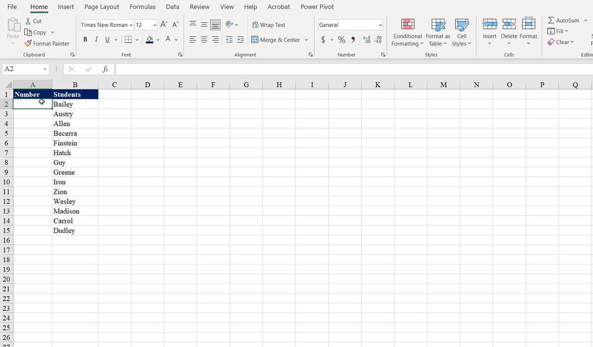
11. SEQUENCE & COUNTA
SEQUENCE returns a sequence of numbers in an array.
COUNTA counts the number of cells in a range that are not empty.
They provide a list where a sequence will continue populating when you add information to the list.
The formula is =SEQUENCE(COUNTA(B:B))
SEQUENCE returns a sequence of numbers in an array.
COUNTA counts the number of cells in a range that are not empty.
They provide a list where a sequence will continue populating when you add information to the list.
The formula is =SEQUENCE(COUNTA(B:B))
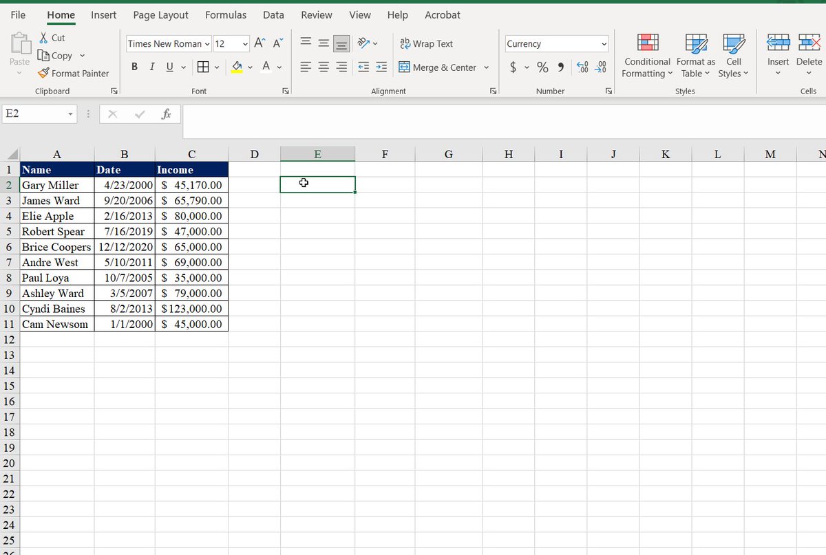
12. SORT
The SORT function sorts the contents of a range or array of data.
We first sorted our table by name, which is the first column.
Then, we sorted by date and income, respectively, by adding the 2 and 3.
The formula is = SORT(A2:C11).
The SORT function sorts the contents of a range or array of data.
We first sorted our table by name, which is the first column.
Then, we sorted by date and income, respectively, by adding the 2 and 3.
The formula is = SORT(A2:C11).
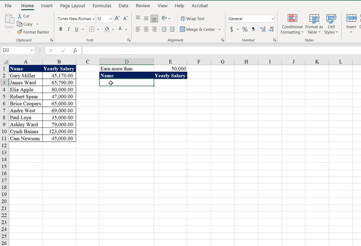
13. FILTER
The FILTER function allows you to filter a range of data based on a defined criterion.
We filtered the results to persons earning more than $50,000.
Then, we sorted their yearly salary in descending order.
The formula is =SORT(FILTER(A2:B11,B2:B11>E1),2,-1).
The FILTER function allows you to filter a range of data based on a defined criterion.
We filtered the results to persons earning more than $50,000.
Then, we sorted their yearly salary in descending order.
The formula is =SORT(FILTER(A2:B11,B2:B11>E1),2,-1).
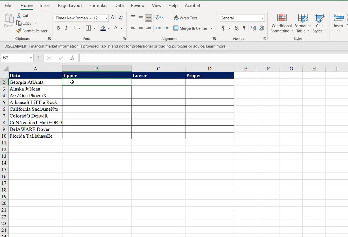
14. UPPER, LOWER, AND PROPER
=UPPER converts a text string to all uppercase.
=LOWER converts a text string to all lowercase.
=PROPER converts a text string to the proper case.
For each of the formulas, we use the information from (A2:A10).
=UPPER converts a text string to all uppercase.
=LOWER converts a text string to all lowercase.
=PROPER converts a text string to the proper case.
For each of the formulas, we use the information from (A2:A10).
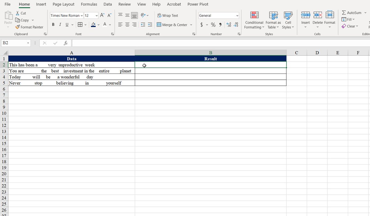
15. TRIM
The TRIM function removes extra spaces from a text string, whether at the beginning, middle, or end.
In the example, we had text strings that had a lot of spaces. When we used the function, the spaces were removed.
The formula is =TRIM(A2).
The TRIM function removes extra spaces from a text string, whether at the beginning, middle, or end.
In the example, we had text strings that had a lot of spaces. When we used the function, the spaces were removed.
The formula is =TRIM(A2).
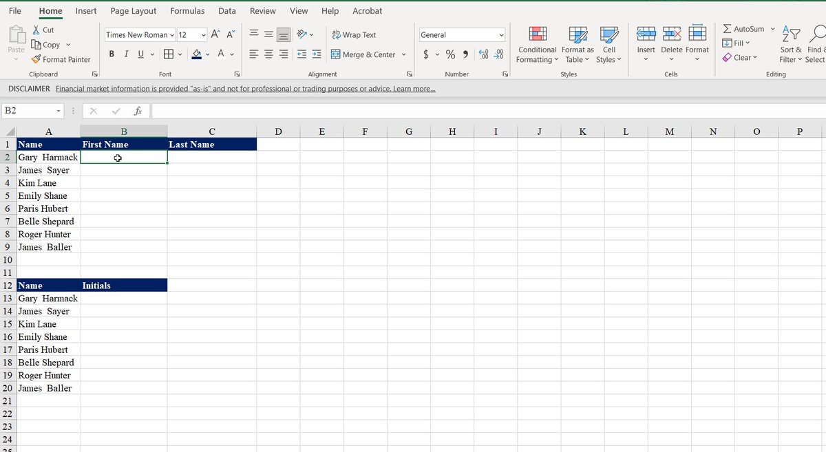
16. Flash Fill
Flash Fill automatically fills your data when it senses a pattern.
Excel detected the pattern and recreated the expected outcome after we input the first name, last name, and initials.
Flash Fill automatically fills your data when it senses a pattern.
Excel detected the pattern and recreated the expected outcome after we input the first name, last name, and initials.
If you enjoyed this thread, please like, comment, and retweet the first tweet.
I write about
- Personal Finance
- Investing
- Wealth
Follow me @AccentInvesting to get more tips.
Subscribe and get a Free guide on 5 ETFs to hold for life: bit.ly
I write about
- Personal Finance
- Investing
- Wealth
Follow me @AccentInvesting to get more tips.
Subscribe and get a Free guide on 5 ETFs to hold for life: bit.ly
Investing in index funds is the simplest way to build wealth.
Start your investing journey today: accentinvesting.gumroad.com
Start your investing journey today: accentinvesting.gumroad.com

Loading suggestions...