

I spent a good portion of my $90,000 master's degree learning 1 thing:
Simulating stock prices.
The good news?
You don't need a master's degree to build your own stock price simulator in Python.
I'm going to show you how step-by-step:
Simulating stock prices.
The good news?
You don't need a master's degree to build your own stock price simulator in Python.
I'm going to show you how step-by-step:
By reading this thread, you'll be able to build your own stock price simulator in Python.
Here's what you'll learn:
1. About Geometric Brownian Motion
2. Import libraries and set up
3. Build the functions
4. Visualize results
Ready?
Here's what you'll learn:
1. About Geometric Brownian Motion
2. Import libraries and set up
3. Build the functions
4. Visualize results
Ready?
A primer:
GBM is a continuous-time stochastic process where the log of the random variable follows the Wiener process with drift.
What?
It’s a data series that trends up or down through time with a defined level of volatility.
And it’s perfect for simulating stock prices.
GBM is a continuous-time stochastic process where the log of the random variable follows the Wiener process with drift.
What?
It’s a data series that trends up or down through time with a defined level of volatility.
And it’s perfect for simulating stock prices.
A Wiener process is a one-dimensional Brownian motion.
It's used in quant finance because of some useful mathematical properties.
In practice, it's used interchangeably with GBM.
You can read more on Wikipedia.
Ok enough, let's see the code!
en.wikipedia.org
It's used in quant finance because of some useful mathematical properties.
In practice, it's used interchangeably with GBM.
You can read more on Wikipedia.
Ok enough, let's see the code!
en.wikipedia.org
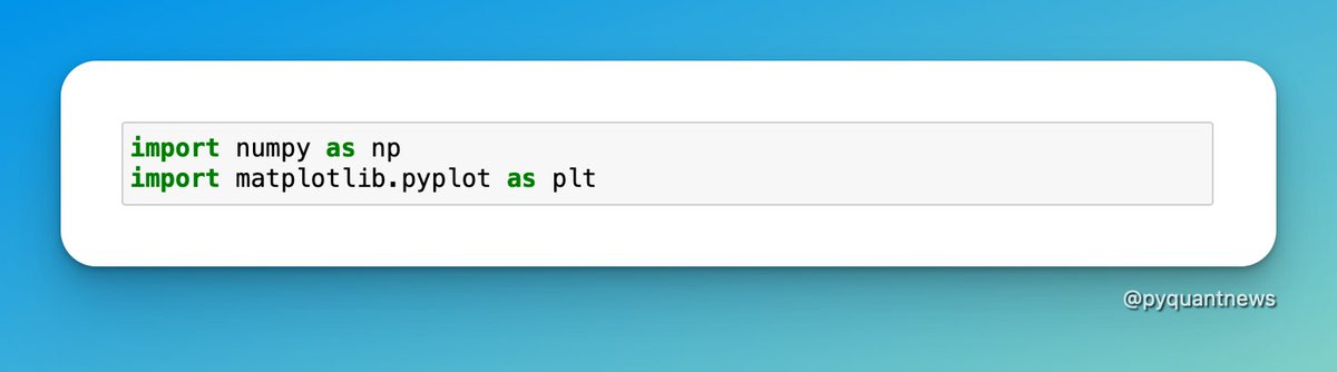
Start by importing the libraries.
Since you're simulating stock prices, you don’t need to download data.
All you need is NumPy for the math and matplotlib for the plots.
Next, set some variables:
Since you're simulating stock prices, you don’t need to download data.
All you need is NumPy for the math and matplotlib for the plots.
Next, set some variables:
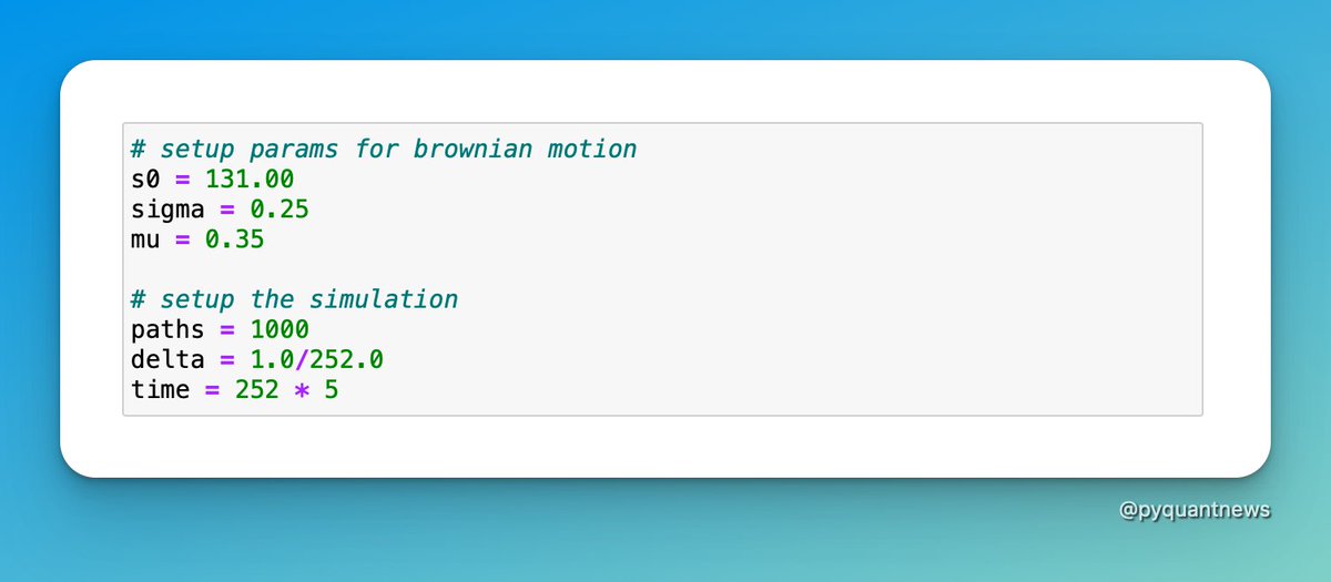
To simulate stock prices, you need to set some input parameters.
Start with these:
• sigma is the percentage volatility
• s0 is the initial stock price
• mu is the trend
This setup will simulate 1,000 paths with daily time steps over 5 years.
Start with these:
• sigma is the percentage volatility
• s0 is the initial stock price
• mu is the trend
This setup will simulate 1,000 paths with daily time steps over 5 years.
The first function returns a Wiener process.
You'll end up with a 2-dimensional NumPy array with 1,260 rows and 1,000 columns.
Each row is a day and each column is a simulation path.
You'll end up with a 2-dimensional NumPy array with 1,260 rows and 1,000 columns.
Each row is a day and each column is a simulation path.

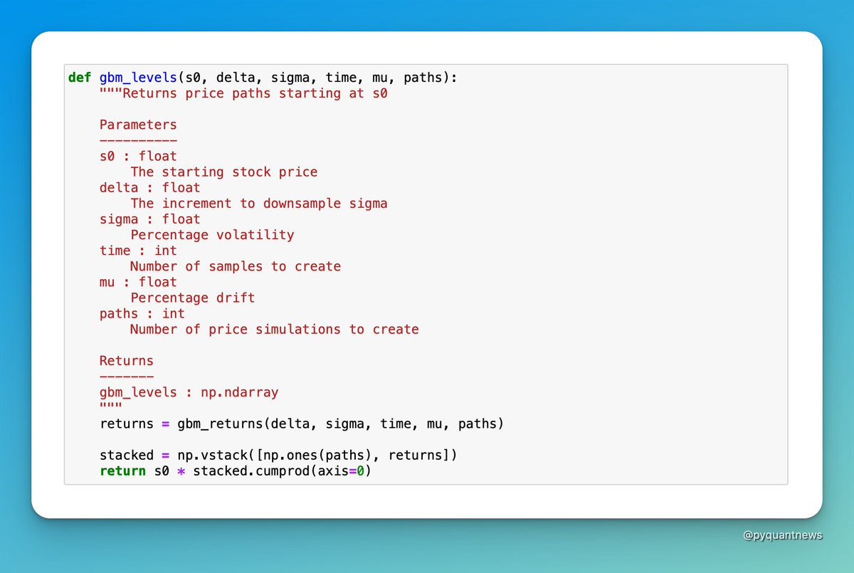
Next, define a function that creates the GBM returns.

Finally, you can build the price paths.
Prepend a row of 1s to the returns array and multiply the starting stock price by the cumulative product of the GBM returns.
Prepend a row of 1s to the returns array and multiply the starting stock price by the cumulative product of the GBM returns.
If this is all a little too abstract, you might like the Ultimate Guide to Pricing Options and Implied Volatility With Python were GBM is used.
• Black-Scholes, the greeks, and implied volatility
• Jupyter Notebooks with the code
• Live options data
pyquantnews.gumroad.com
• Black-Scholes, the greeks, and implied volatility
• Jupyter Notebooks with the code
• Live options data
pyquantnews.gumroad.com
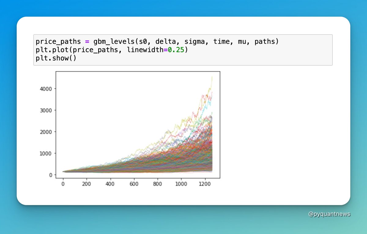
You can look at 2 examples.
The first simulates 1,000 price paths over 5 years.
It starts at a price of 131 with 25% volatility and 35% return.
(This is the volatility and return of Apple in 2021.)
A 35% drift causes most price paths to increase from the initial price.
The first simulates 1,000 price paths over 5 years.
It starts at a price of 131 with 25% volatility and 35% return.
(This is the volatility and return of Apple in 2021.)
A 35% drift causes most price paths to increase from the initial price.
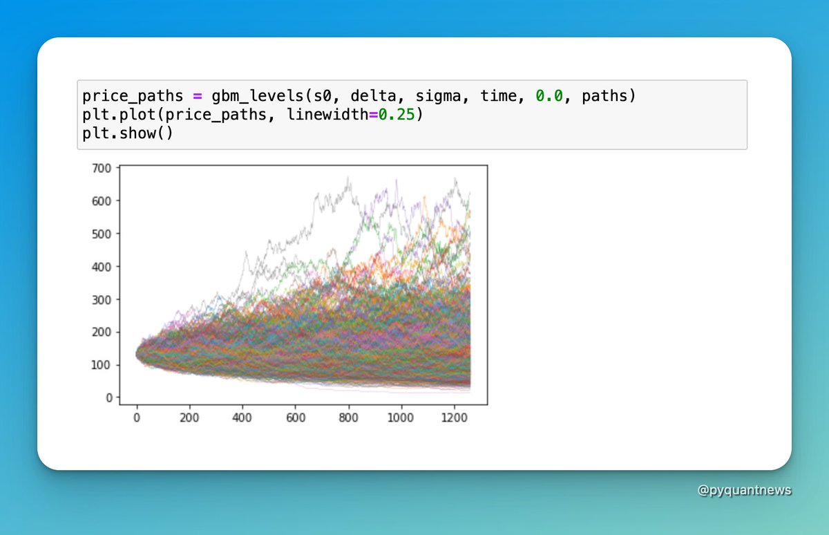
In the second example, set the drift to 0.0.
Only about half the prices end up higher than the original price.
Does this make sense?
Since the source of randomness is a variable from a normal distribution, it makes sense that half the values lie on either side of the mean.
Only about half the prices end up higher than the original price.
Does this make sense?
Since the source of randomness is a variable from a normal distribution, it makes sense that half the values lie on either side of the mean.
Spend some time and play around with the variables.
• What happens if you double volatility?
• What happens if you set mu to a negative number?
You can use this code to simulate a trading strategy too.
It's a great way to get some intuition about how markets behave.
• What happens if you double volatility?
• What happens if you set mu to a negative number?
You can use this code to simulate a trading strategy too.
It's a great way to get some intuition about how markets behave.
I really hope you enjoyed this thread.
If there's too much to consume now, retweet the top tweet so you can find it later.
You can also follow me @pyquantnews for more tweets and threads that help you get started with Python for quant finance.
If there's too much to consume now, retweet the top tweet so you can find it later.
You can also follow me @pyquantnews for more tweets and threads that help you get started with Python for quant finance.
If you like Tweets performance metrics in your trading, you might enjoy my weekly newsletter: The PyQuant Newsletter.
Python code for quantitative analysis you can use.
Join 4,600+ subscribers who are taking action with Python.
pyquantnews.com
Python code for quantitative analysis you can use.
Join 4,600+ subscribers who are taking action with Python.
pyquantnews.com
Loading suggestions...