

You’ve likely heard of the term “impermanent loss” before but what does it mean, why is it significant and what’s with the quotations? 😂
A 🧵on everything you wanted to know regarding IL👇
A 🧵on everything you wanted to know regarding IL👇
Before we dive in, give our previous 🧵a quick read. It explains the return profiles of CFMMs like UniV2, Sushiswap, etc.
With the ability to derive returns & IL, one can accurately estimate the EV of depositing into a pool.
1/n
With the ability to derive returns & IL, one can accurately estimate the EV of depositing into a pool.
1/n
Now, let’s start by defining “impermanent loss”. The reason for the quotations is that the term is a misnomer.
The loss is not an actual loss LPs experience, but rather, an opportunity cost.
2/n
The loss is not an actual loss LPs experience, but rather, an opportunity cost.
2/n
It is the difference between the value of the stake in the pool & the value of the stake had it been HODLd, excluding trading fees.
As the reserve ratio changes, the LP position always underperforms the stake not invested in the pool. IL increases w greater price changes.
3/n
As the reserve ratio changes, the LP position always underperforms the stake not invested in the pool. IL increases w greater price changes.
3/n
Since the goal of measuring IL is to estimate opportunity cost, we will ignore trading fees.
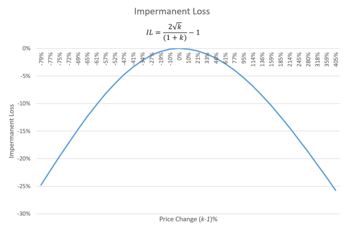
Formula for IL:
IL = (V₁ - Vₕ) / Vₕ = 2√k / (1 + k) - 1
where k is a number from 0 to ∞ representing the change in price from the original LP position. H means held in spot
4/n
Formula for IL:
IL = (V₁ - Vₕ) / Vₕ = 2√k / (1 + k) - 1
where k is a number from 0 to ∞ representing the change in price from the original LP position. H means held in spot
4/n
To derive the IL function, we have to define a formula for the value of the liquidity stake had it not been supplied to the pool.
First, create a future price variable p’ which is equal to p*k. p is the initial price of liquidity provided and k is a number within 0 and ∞
5/n
First, create a future price variable p’ which is equal to p*k. p is the initial price of liquidity provided and k is a number within 0 and ∞
5/n
p’ = p * k
then using the formula defined for the value of the stake in the pool with p’ instead, we derive the following
Vₕ = x * p’ + y = (L * p * k)/√p + L√p = L√p * k + L√p
when simplifying the formula we get
Vₕ = L√p * (1+k)
6/n
then using the formula defined for the value of the stake in the pool with p’ instead, we derive the following
Vₕ = x * p’ + y = (L * p * k)/√p + L√p = L√p * k + L√p
when simplifying the formula we get
Vₕ = L√p * (1+k)
6/n
Now we plug in p’ for the value of the LP position to derive the formula as a function of k, the value of the LP position in the next timestep.
V₁ = 2L√p’ = 2L√(p * k)
7/n
V₁ = 2L√p’ = 2L√(p * k)
7/n
Finally, to derive IL we subtract the difference in value of the stake as a % of the stake that was not invested in the pool
IL(k) = (V₁ - Vₕ) / Vₕ = L√p * (2√k -1 -k) / L√p * (1 + k) = 2√k / (1+k) - 1z
As shown, IL increases as the price deviates from the original.
8/n
IL(k) = (V₁ - Vₕ) / Vₕ = L√p * (2√k -1 -k) / L√p * (1 + k) = 2√k / (1+k) - 1z
As shown, IL increases as the price deviates from the original.
8/n
It it called impermanent loss because if the price ever reverts back to the original price at which liquidity was provided, the loss disappears.
IL is important bc it lets us estimate the potential underperformance of LPing / EV
9/n
IL is important bc it lets us estimate the potential underperformance of LPing / EV
9/n
However, IL cannot be the only metric one takes into consideration, since a liquidity pool also earns trading fees.
Therefore, one must add fees to the return function of the LP to measure real performance.
10/n
Therefore, one must add fees to the return function of the LP to measure real performance.
10/n
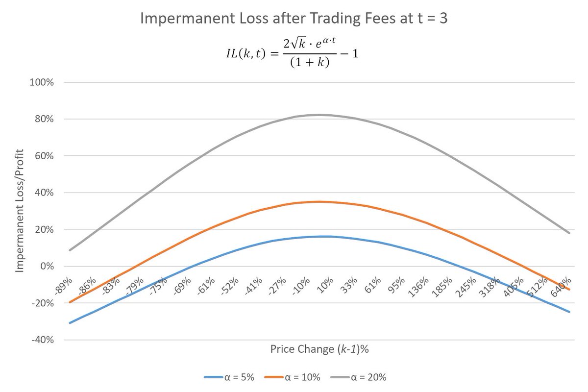
To add trading fees, we substitute the formula for the value of the LP including fees for the value of the stake in the pool excluding fees in the IL equation,
IL(k,t) = (V₁ - Vₕ) / Vₕ = 2L√(p*k)*e^(α*t) - L√p(1+k) / L√p(1+K)
After simplication, we get 👇
11/n
IL(k,t) = (V₁ - Vₕ) / Vₕ = 2L√(p*k)*e^(α*t) - L√p(1+k) / L√p(1+K)
After simplication, we get 👇
11/n
IL(k,t) = 2√k * e^(α*t) / (1 + k) - 1
As you can see, trading fees can substantially remediate underperformance of IL or even lead to outperformance.
The problem with fees is that they are not necessarily correlated with vol. More on that in a future 🧵👀
12/n
As you can see, trading fees can substantially remediate underperformance of IL or even lead to outperformance.
The problem with fees is that they are not necessarily correlated with vol. More on that in a future 🧵👀
12/n
Trading fees can add substantial upside and even compensate you fully for your IL.
Unfortunately, the effect of fees decreases as price deviates from the original price of the LP in V2 models. This is due to the sqrt relationship between returns and price inside AMMs.
13/n
Unfortunately, the effect of fees decreases as price deviates from the original price of the LP in V2 models. This is due to the sqrt relationship between returns and price inside AMMs.
13/n
Although AMMs are described as market makers, their returns profiles are uniquely different to that of traditional firms. Tradfi MMs hedge price variation and limit their returns to the bid ask spread of the markets they make.
LPs carry substantial inventory risk though.
14/n
LPs carry substantial inventory risk though.
14/n
The risk is unhedged product the LP is carrying in their book.
Therefore, a rational LP is betting that the trading fees they collect will be greater than the losses from price declines and greater than the underperformance from IL
15/n
Therefore, a rational LP is betting that the trading fees they collect will be greater than the losses from price declines and greater than the underperformance from IL
15/n
This exposure to losses from price declining negatively skews the potential returns of liquidity pools and unless done correctly is a -EV trade.
In the next 🧵, we will introduce a way to hedge away market risk and drive more consistent returns.
16/n
In the next 🧵, we will introduce a way to hedge away market risk and drive more consistent returns.
16/n
Conclusion: Taking into account the return formula from last thread, Rₜ = √Pₜe^(α*t) - 1, and the formula for IL we derived in this thread, one can accurately estimate the EV of an LP position.
If you enjoyed
1) Drop a 👍 & RT
2) Turn on 🐦 notifications
17/n
If you enjoyed
1) Drop a 👍 & RT
2) Turn on 🐦 notifications
17/n
Loading suggestions...