
Technology
Artificial Intelligence
Computer Science
Machine Learning
Neural Networks
Optimization Algorithms

The batch size is one of the most influential parameters in the outcome of a neural network.
Here is everything you need to know about the batch size when training a neural network:
1 of 18
Here is everything you need to know about the batch size when training a neural network:
1 of 18

Gradient Descent is an optimization algorithm to train neural networks.
The algorithm computes how much we need to adjust the model to get closer to the desired results on every iteration.
Here is how it works in a couple of sentences:
3 of 18
The algorithm computes how much we need to adjust the model to get closer to the desired results on every iteration.
Here is how it works in a couple of sentences:
3 of 18
We take samples from the training dataset, run them through the model, and determine how far away our results are from the ones we expect.
We use this "error" to compute how much we need to update the model weights to improve the results.
4 of 18
We use this "error" to compute how much we need to update the model weights to improve the results.
4 of 18
A critical decision we need to make is how many samples we use on every iteration.
We have three choices:
• Use a single sample of data
• Use all of the data at once
• Use some of the data
5 of 18
We have three choices:
• Use a single sample of data
• Use all of the data at once
• Use some of the data
5 of 18
Using a single sample of data on every iteration is called "Stochastic Gradient Descent" (SGD.)
The algorithm uses one sample at a time to compute the updates.
6 of 18
The algorithm uses one sample at a time to compute the updates.
6 of 18
Advantages of Stochastic Gradient Descent:
• Simple to understand
• Avoids getting stuck in local minima
• Provides immediate feedback
Disadvantages:
• Computationally intensive
• May not settle in the global minimum
• The performance will be noisy
7 of 18
• Simple to understand
• Avoids getting stuck in local minima
• Provides immediate feedback
Disadvantages:
• Computationally intensive
• May not settle in the global minimum
• The performance will be noisy
7 of 18
Using all the data at once is called "Batch Gradient Descent."
After processing every sample, the algorithm takes the entire dataset and computes the updates.
8 of 18
After processing every sample, the algorithm takes the entire dataset and computes the updates.
8 of 18
Advantages of Batch Gradient Descent:
• Computationally efficient
• Stable performance (less noise)
Disadvantages:
• Requires a lot of memory
• May get stuck in local minima
9 of 18
• Computationally efficient
• Stable performance (less noise)
Disadvantages:
• Requires a lot of memory
• May get stuck in local minima
9 of 18
Using some data (more than one sample but fewer than the entire dataset) is called "Mini-Batch Gradient Descent."
The algorithm works like Batch Gradient Descent, the only difference being that we use fewer samples.
10 of 18
The algorithm works like Batch Gradient Descent, the only difference being that we use fewer samples.
10 of 18
Advantages of Mini-Batch Gradient Descent:
• Avoids getting stuck in local minima
• More computationally efficient than SGD
• Doesn't need as much memory as BGD
Disadvantages:
• New hyperparameter to worry about
We usually call this hyperparameter "batch_size."
11 of 18
• Avoids getting stuck in local minima
• More computationally efficient than SGD
• Doesn't need as much memory as BGD
Disadvantages:
• New hyperparameter to worry about
We usually call this hyperparameter "batch_size."
11 of 18
We rarely use Batch Gradient Descent in practice, especially with large datasets.
Stochastic Gradient Descent (using a single sample at a time) is not that popular either.
Mini-Batch is the most used.
12 of 18
Stochastic Gradient Descent (using a single sample at a time) is not that popular either.
Mini-Batch is the most used.
12 of 18
There's a lot of research around the optimal batch size.
Your problem differs from any other problem, but empirical evidence suggests that smaller batches perform better.
(Small as in less than a hundred or so.)
13 of 18
Your problem differs from any other problem, but empirical evidence suggests that smaller batches perform better.
(Small as in less than a hundred or so.)
13 of 18
I created a notebook to train a neural network in three different ways:
1. Using batch size = 1
2. Using batch size = 32
3. Using batch size = n
colab.research.google.com
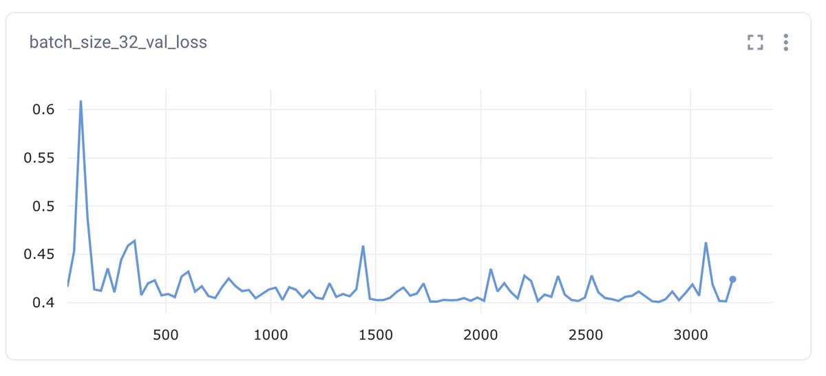
Attached you can see how the accuracy moved in each of these experiments:
15 of 18
1. Using batch size = 1
2. Using batch size = 32
3. Using batch size = n
colab.research.google.com
Attached you can see how the accuracy moved in each of these experiments:
15 of 18
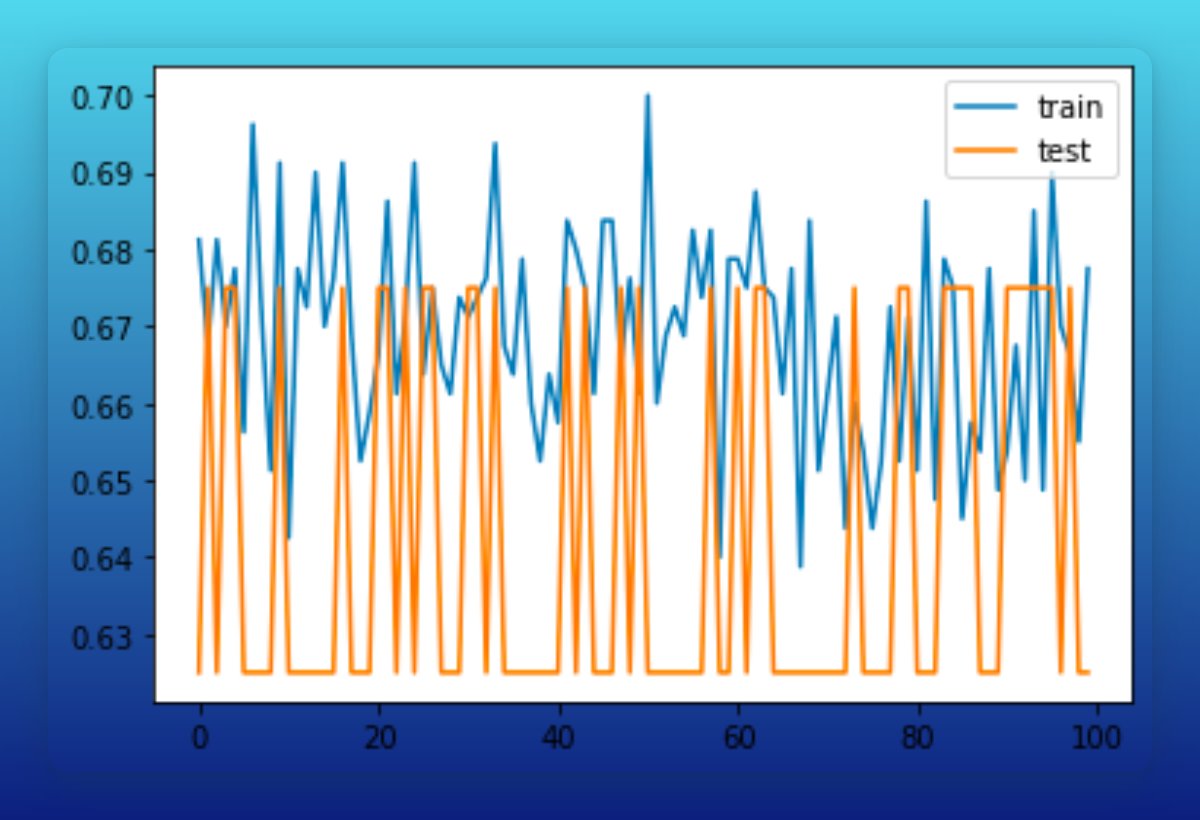

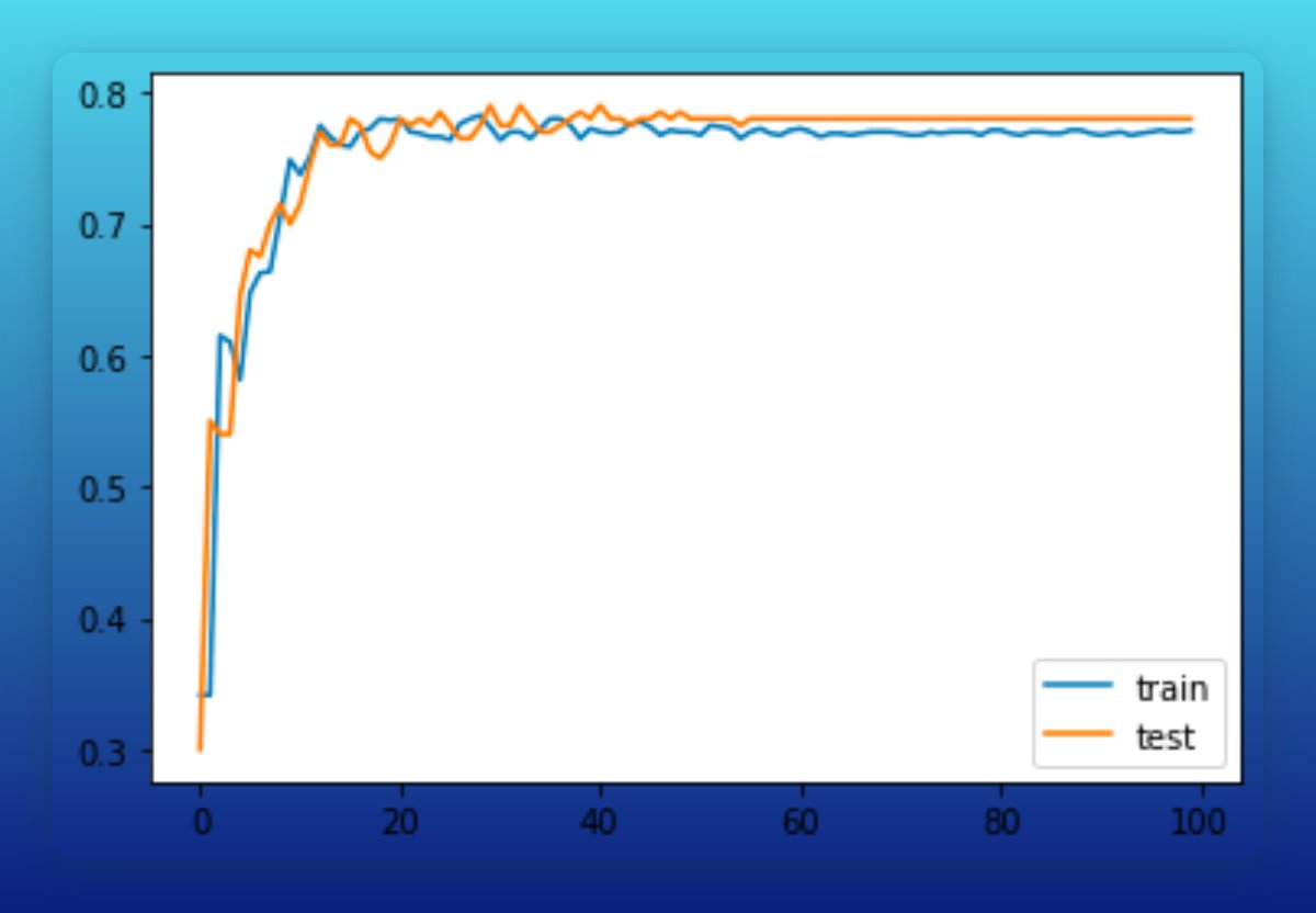
A few notes:
• Training time: 263s, 21s, and 8s, respectively.
• Testing accuracy: 0.62, 0.77, 0.78, respectively.
• Attached images show the noise in the testing loss.
Noticeable differences!
16 of 18
• Training time: 263s, 21s, and 8s, respectively.
• Testing accuracy: 0.62, 0.77, 0.78, respectively.
• Attached images show the noise in the testing loss.
Noticeable differences!
16 of 18


Every week, I break down machine learning concepts to give you ideas on applying them in real-life situations.
Follow me @svpino to ensure you don't miss what's coming next.
18 of 18
Follow me @svpino to ensure you don't miss what's coming next.
18 of 18
Loading suggestions...