

I've built many financial models in Excel while working at Goldman Sachs & JP Morgan.
1 Billion others use Microsoft Excel, it's the most valuable skill in many careers.
🧵Here are 10 Excel functions everyone should master:
1 Billion others use Microsoft Excel, it's the most valuable skill in many careers.
🧵Here are 10 Excel functions everyone should master:
Here are 12 MUST-KNOW Microsoft Excel functions:
(1) XLOOKUP
(2) Wildcards
(3) Sparklines
(4) Filter
(5) Pivot Tables
(6) IF
(7) SUMIFS
(8) COUNTIFS
(9) Transpose
(10) TRIM
Let's discuss each with examples:
(1) XLOOKUP
(2) Wildcards
(3) Sparklines
(4) Filter
(5) Pivot Tables
(6) IF
(7) SUMIFS
(8) COUNTIFS
(9) Transpose
(10) TRIM
Let's discuss each with examples:
(1) XLOOKUP:
XLookup is an upgrade compared to VLOOKUP or Index & Match.
Use the XLOOKUP function to find things in a table or range by row.
Formula: =XLOOKUP (lookup value, lookup array, return array)
XLookup is an upgrade compared to VLOOKUP or Index & Match.
Use the XLOOKUP function to find things in a table or range by row.
Formula: =XLOOKUP (lookup value, lookup array, return array)

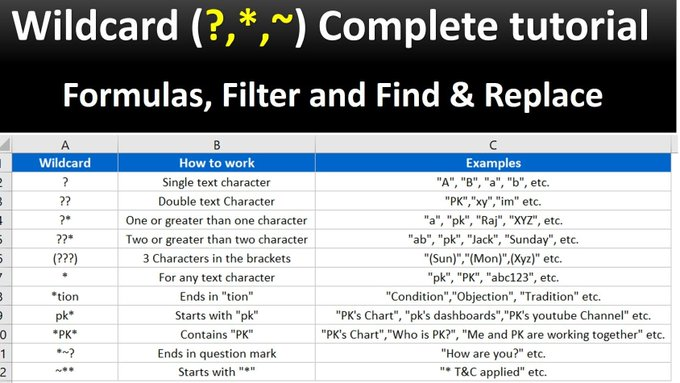
(2) Wildcards:
A wildcard is a special character that allows you to perform partial matches in your Excel formulas.
Excel has three wildcards:
• asterisk "*"
• question mark "?"
• tilde "~"
A wildcard is a special character that allows you to perform partial matches in your Excel formulas.
Excel has three wildcards:
• asterisk "*"
• question mark "?"
• tilde "~"
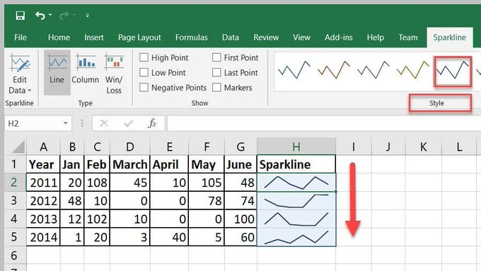
(3) Sparklines:
Sparklines allow you to insert mini graphs inside a cell to provide a visual representation of data.
Use sparklines to show trends or patterns in data.
On the 'Insert tab', click 'Sparklines'
Sparklines allow you to insert mini graphs inside a cell to provide a visual representation of data.
Use sparklines to show trends or patterns in data.
On the 'Insert tab', click 'Sparklines'
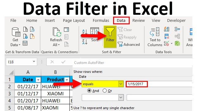
(4) Filter:
The FILTER function allows you to filter data based on a query.
For example, you can filter a column to show a specific product or date.
You can also sort in ascending or descending order.
The shortcut for this function is CTRL + SHFT + L
The FILTER function allows you to filter data based on a query.
For example, you can filter a column to show a specific product or date.
You can also sort in ascending or descending order.
The shortcut for this function is CTRL + SHFT + L
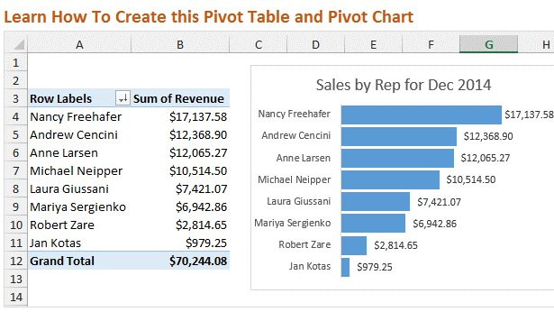
(5) Pivot Tables:
A powerful tool to calculate, summarize & analyze data, which allows you to compare or find patterns & trends in data.
To access this function, go to "Insert" in the Menu bar, and then select "Pivot Table"
A powerful tool to calculate, summarize & analyze data, which allows you to compare or find patterns & trends in data.
To access this function, go to "Insert" in the Menu bar, and then select "Pivot Table"
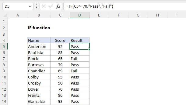
(6) IF:
The IF function makes logical comparisons & tells you when certain conditions are met.
For example, a logical comparison would be to return the word "Pass" if a score is >70, and if not, it will say "Fail"
An example of this formula would be =IF(C5>70,"Pass","Fail")
The IF function makes logical comparisons & tells you when certain conditions are met.
For example, a logical comparison would be to return the word "Pass" if a score is >70, and if not, it will say "Fail"
An example of this formula would be =IF(C5>70,"Pass","Fail")
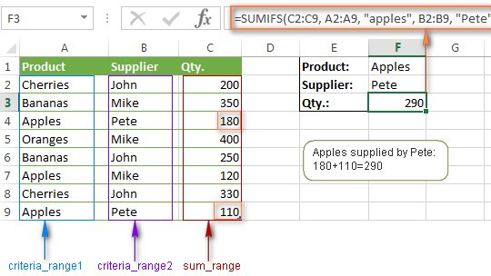
(7) SUMIFS:
SUMIFS sum the values in a range that meet multiple criteria.
For example, use it if you want the sum of two criteria, for example, Apples from Pete.
The formula is SUMIFS (sum_range, criteria_range1, criteria1, [criteria_range2, criteria2], ...)
SUMIFS sum the values in a range that meet multiple criteria.
For example, use it if you want the sum of two criteria, for example, Apples from Pete.
The formula is SUMIFS (sum_range, criteria_range1, criteria1, [criteria_range2, criteria2], ...)
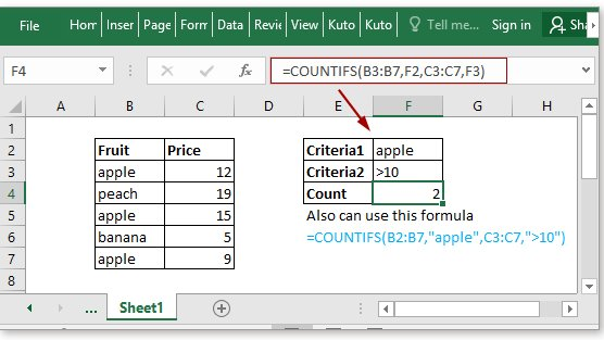
(8) COUNTIFS:
CountIf counts the number of times a criteria is met.
For example, it counts the number of times that both (1) apples and (2) price > $10, are mentioned.
CountIf counts the number of times a criteria is met.
For example, it counts the number of times that both (1) apples and (2) price > $10, are mentioned.
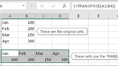
(9) Transpose:
This will transform items in rows, to instead be shown in columns or vice versa.
To transpose a column to a row:
• Select the data in the column
• Select the cell you want the row to start
• Right click, choose to paste special, select transpose
This will transform items in rows, to instead be shown in columns or vice versa.
To transpose a column to a row:
• Select the data in the column
• Select the cell you want the row to start
• Right click, choose to paste special, select transpose
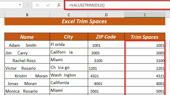
(10) TRIM:
TRIM removes the extra spaces in data.
TRIM can be useful in removing irregular spacing from imported data
=TRIM()
TRIM removes the extra spaces in data.
TRIM can be useful in removing irregular spacing from imported data
=TRIM()
BONUS:
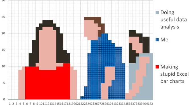
You can use Microsoft Excel to create art:
You can use Microsoft Excel to create art:
These 10 Excel functions will make you an expert & increase your productivity by 100X
If you found this thread helpful:
• Follow me @FluentInFinance
•🔁RT the FIRST tweet
• Sign-up for my FREE newsletter to learn valuable skills: FluentInFinance.Substack.com!
If you found this thread helpful:
• Follow me @FluentInFinance
•🔁RT the FIRST tweet
• Sign-up for my FREE newsletter to learn valuable skills: FluentInFinance.Substack.com!

Loading suggestions...