

There is $482,000,000,000 invested in factor ETFs.
Factors can help you diversify risk and drive returns.
Unfortunately, most people don’t know how.
Until now.
Here’s a step-by-step guide for doing it in Python:
Factors can help you diversify risk and drive returns.
Unfortunately, most people don’t know how.
Until now.
Here’s a step-by-step guide for doing it in Python:
By reading this thread, you’ll be able to:
• Download historic factor data
• Compute the sensitivities to the factors
• Figure out the risk contribution of the factors
But first…
• Download historic factor data
• Compute the sensitivities to the factors
• Figure out the risk contribution of the factors
But first…
A quick primer on factor investing:
• Used to target specific return drivers
• Helps manage risk outside diversification
• Important for active managers that get paid for performance
You can use the famous Fama-French 3-factor model for free.
Here’s how:
• Used to target specific return drivers
• Helps manage risk outside diversification
• Important for active managers that get paid for performance
You can use the famous Fama-French 3-factor model for free.
Here’s how:
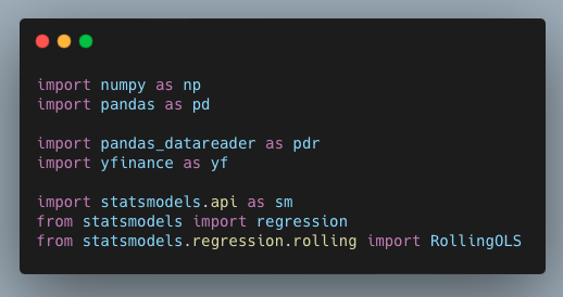
First, import the libraries.
You can use pandas_datareader to download the factor data and yfinance to download stock price data.
Use `statsmodels` for modeling.
You can use pandas_datareader to download the factor data and yfinance to download stock price data.
Use `statsmodels` for modeling.
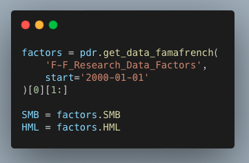
`MB is “small minus big” representing the size factor.
HML is “high minus low” representing the style factor.
This also downloads the third factor, `Rm-Rf`, which is the portfolio excess return.
I only use `SMB` and `HML` for this analysis.
HML is “high minus low” representing the style factor.
This also downloads the third factor, `Rm-Rf`, which is the portfolio excess return.
I only use `SMB` and `HML` for this analysis.
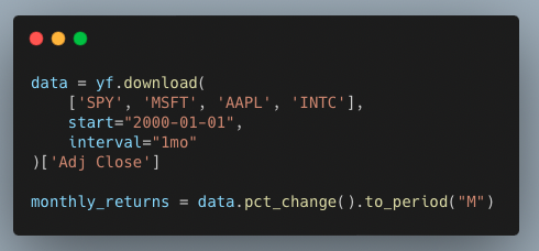
Now get the stock data for your portfolio.
You can pick any stocks you want.
(Make sure to include a benchmark list SPY.)
Get monthly closing prices and resample to monthly labels to align with the factor data.
You can pick any stocks you want.
(Make sure to include a benchmark list SPY.)
Get monthly closing prices and resample to monthly labels to align with the factor data.
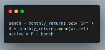
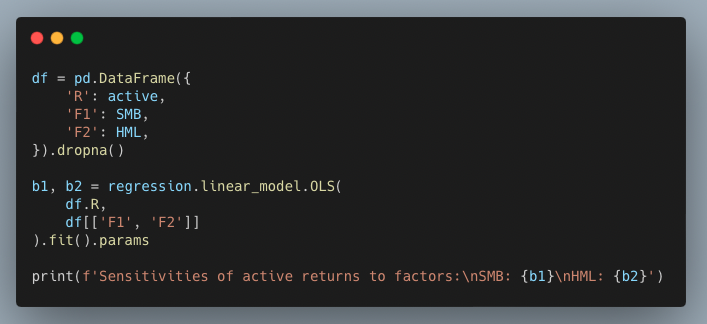
Next, you will compute the active return of the portfolio.
The active return is the portfolio return minus the benchmark return.
The active return is the portfolio return minus the benchmark return.
Run a regression with the active returns as the variable dependent on the factors.
Fitting the model gives you the two coefficients that determine the sensitivities of the portfolio’s active returns to the factors.
Fitting the model gives you the two coefficients that determine the sensitivities of the portfolio’s active returns to the factors.
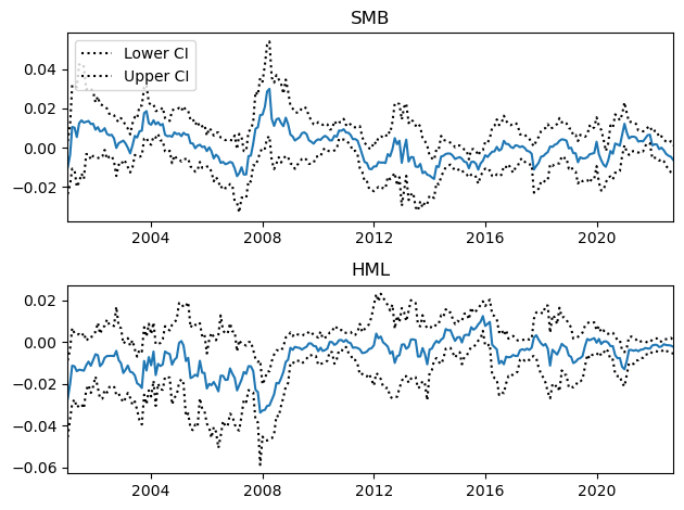
The sensitivities are estimates so it’s important to see how they evolve through time.
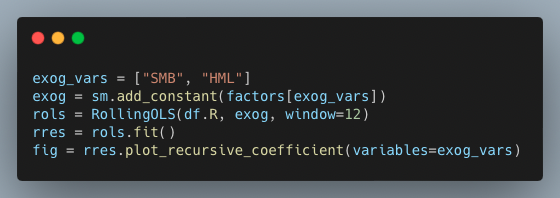
The dashed lines are confidence intervals around the beta estimates.
Marginal Contribution To Active Risk (MCTAR) measures the incremental risk each additional factor introduces to your portfolio.
You'll see how to compute it next:
You'll see how to compute it next:
To figure out the factor’s MCTAR, multiply the factor sensitivity by the covariance between the two factors.
Then divide by the standard deviation of the active returns, squared.
Then divide by the standard deviation of the active returns, squared.
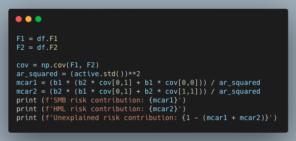
MCTAR tells you how much risk you take on by being exposed to each factor given the other factors you’re already exposed to.
The unexplained risk contribution is the exposure you have to other factors outside of the two you analyzed.
The unexplained risk contribution is the exposure you have to other factors outside of the two you analyzed.
Now you can:
• Download historic factor data
• Compute the sensitivities to the factors
• Figure out the risk contribution of the factors
Use this analysis to manage risk in your own portfolio.
• Download historic factor data
• Compute the sensitivities to the factors
• Figure out the risk contribution of the factors
Use this analysis to manage risk in your own portfolio.
There's a lot here!
Want to keep this guide handy?
Hop back to the top and retweet the top tweet so you can find it later - and so others can find it too!
Here's the link:
Want to keep this guide handy?
Hop back to the top and retweet the top tweet so you can find it later - and so others can find it too!
Here's the link:
The FREE 7-day masterclass that will get you up and running with Python for quant finance.
Here's what you get:
• Working code to trade with Python
• Frameworks to get you started TODAY
• Trading strategy formation framework
7 days. Big results.
pythonforquantfinancemasterclass.com
Here's what you get:
• Working code to trade with Python
• Frameworks to get you started TODAY
• Trading strategy formation framework
7 days. Big results.
pythonforquantfinancemasterclass.com
Loading suggestions...