

✅ Principal Component Analysis ( PCA) is an important technique in ML - Explained in simple terms.
A quick thread 👇🏻🧵
#MachineLearning #Coding #100DaysofCode #deeplearning #DataScience
PC : Research Gate
A quick thread 👇🏻🧵
#MachineLearning #Coding #100DaysofCode #deeplearning #DataScience
PC : Research Gate

1/ PCA is a linear transformation method that aims to reduce dimensionality of dataset while preserving as much of original variance. It does this by identifying a new set of uncorrelated variables, called principal components, that are linear combinations of original features.

2/ When to use PCA -
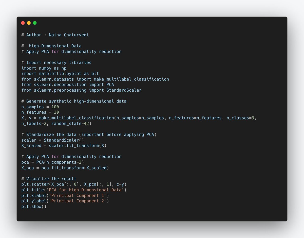
High-Dimensional Data: PCA is especially useful when dealing with high-dimensional datasets, where the number of features (dimensions) is relatively large compared to the number of data points. High dimensionality can lead to various issues.
High-Dimensional Data: PCA is especially useful when dealing with high-dimensional datasets, where the number of features (dimensions) is relatively large compared to the number of data points. High dimensionality can lead to various issues.
3/ Multicollinearity: If your dataset contains highly correlated features (multicollinearity), PCA can help by transforming them into a set of orthogonal (uncorrelated) principal components. This can improve model stability and interpretability.

4/ Data Compression: PCA can be used for data compression, particularly when storage space or bandwidth is limited. By reducing the dimensionality, you can represent data more efficiently while retaining most of its essential characteristics.

5/ Visualization: When you want to visualize high-dimensional data in two or three dimensions, PCA can be used to project the data onto a lower-dimensional space while preserving as much variance as possible. This makes it easier to explore and understand the data.

6/ Why to Use PCA:
Reduced Dimensionality: PCA simplifies the dataset by reducing the number of dimensions. This simplification can lead to faster training and testing of machine learning models, especially when the original feature space is large.
Reduced Dimensionality: PCA simplifies the dataset by reducing the number of dimensions. This simplification can lead to faster training and testing of machine learning models, especially when the original feature space is large.

7/ Noise Reduction: High-dimensional data often contains noise or irrelevant information. PCA can help filter out this noise by focusing on the principal components, which capture the most important patterns in the data.

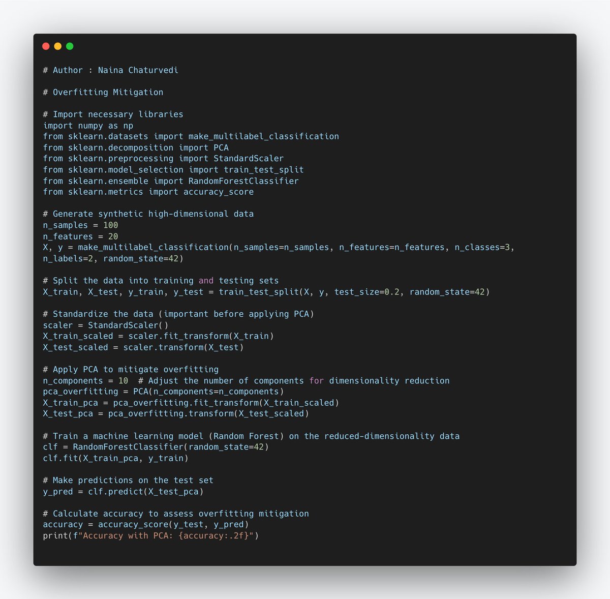
8/ Overfitting Mitigation: PCA reduces the risk of overfitting by decreasing the number of features. Overfitting occurs when a model learns to fit the noise in the data, and by reducing dimensionality, there is less noise to fit.
9/ PCA is a statistical method used for reducing the dimensionality of data while retaining its essential information. It achieves this by identifying the most significant patterns (principal components) in the data and representing it in a lower-dimensional space.
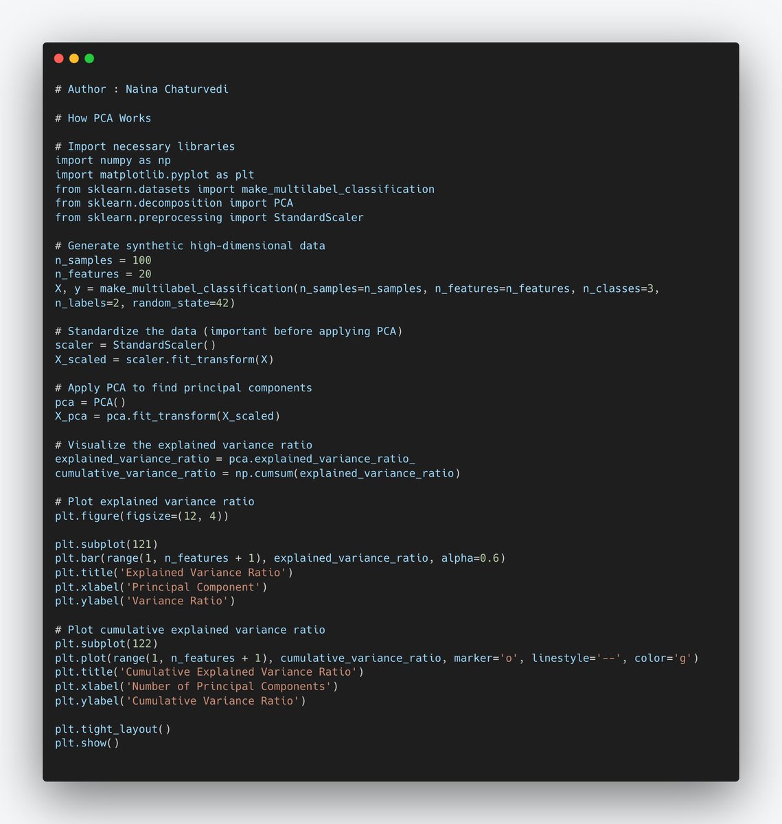
10/ How PCA Works: PCA finds linear combinations of the original features to create new variables (principal components) that maximize the variance in the data. The first principal component captures the most variance, the second captures the second most, and so on.
11/ By selecting a subset of these principal components, you can represent the data with reduced dimensions.
12/ Covariance Matrix:
PCA begins by computing the covariance matrix of the original data. The covariance between two features measures how they change together. A positive covariance indicates that as one feature increases, the other tends to increase as well, and vice versa.
PCA begins by computing the covariance matrix of the original data. The covariance between two features measures how they change together. A positive covariance indicates that as one feature increases, the other tends to increase as well, and vice versa.

13/Eigenvalues and Eigenvectors:
After obtaining the covariance matrix, PCA calculates its eigenvalues and corresponding eigenvectors. Eigenvectors are directions in the original feature space, and eigenvalues represent the variance of data along those directions.
After obtaining the covariance matrix, PCA calculates its eigenvalues and corresponding eigenvectors. Eigenvectors are directions in the original feature space, and eigenvalues represent the variance of data along those directions.

14/ The eigenvector with the highest eigenvalue is the first principal component, the second highest eigenvalue corresponds to the second principal component, and so on. Eigenvalues indicate how much variance is explained by each principal component.
15/ PCA transforms the original features into a new set of orthogonal components (principal components) that capture the maximum variance in the data.

16/ Data Standardization: PCA typically starts with standardizing the data, ensuring that each feature has a mean of 0 and a standard deviation of 1. This step is crucial for PCA to work correctly because it assumes that the data is centered.

17/ Selecting Principal Components: PCA sorts the eigenvalues in descending order. The eigenvector corresponding to the largest eigenvalue becomes the first principal component, the second-largest eigenvalue corresponds to the second principal component, and so on.

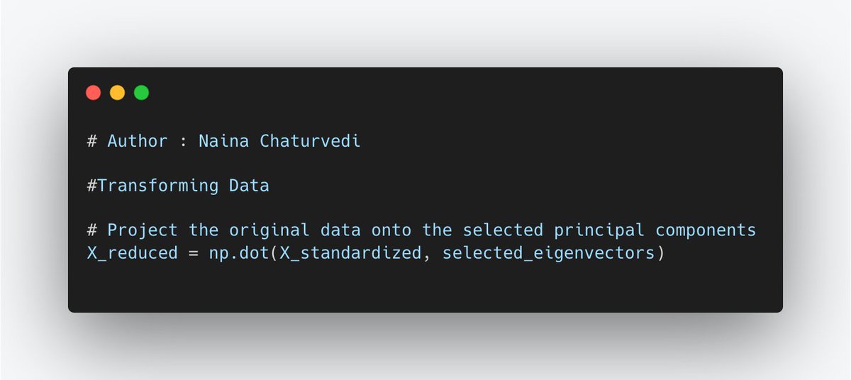
18/ Transforming Data: Finally, the original data is projected onto the selected principal components to create a new dataset with reduced dimensions. This projection is done by taking the dot product of the data and the principal component matrix.
19/ PCA involves a trade-off between reducing dimensionality and retaining information.
Retaining more PCs preserves more information but may result in higher-dimensional data. Reducing the number of retained PCs simplifies the data but may result in information loss.
Retaining more PCs preserves more information but may result in higher-dimensional data. Reducing the number of retained PCs simplifies the data but may result in information loss.

20/ Choosing the Right Number of Principal Components:
Choosing the optimal number of principal components (PCs) to retain in PCA is a crucial decision, as it balances dimensionality reduction with information retention.
Choosing the optimal number of principal components (PCs) to retain in PCA is a crucial decision, as it balances dimensionality reduction with information retention.
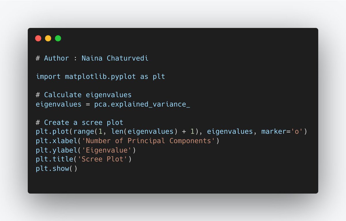
21/ A scree plot is a graphical representation of the eigenvalues (variance) of each principal component, sorted in descending order.
Look for an "elbow" point in scree plot, where eigenvalues start to level off. The number of PCs just before this point is a reasonable choice.
Look for an "elbow" point in scree plot, where eigenvalues start to level off. The number of PCs just before this point is a reasonable choice.
22/ The cumulative explained variance represents the total variance explained by a given number of PCs.
How to Use: Calculate the cumulative explained variance and choose the number of PCs that capture a sufficiently high proportion of the total variance (e.g., 95%).
How to Use: Calculate the cumulative explained variance and choose the number of PCs that capture a sufficiently high proportion of the total variance (e.g., 95%).

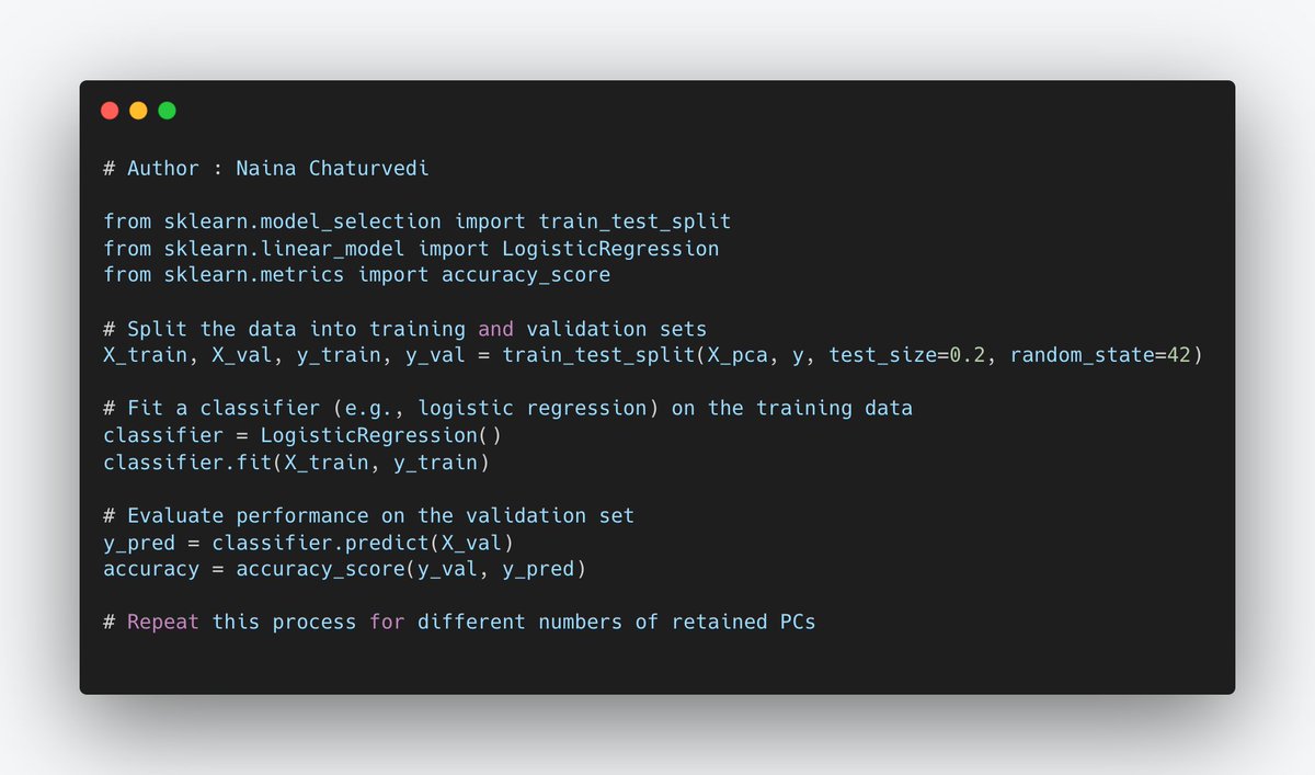
23/ Cross-validation techniques can be used to assess model performance for different numbers of retained PCs.
Split the data into training and validation sets, fit a PCA model with a specific number of PCs on training set, and evaluate its performance on the validation set.
Split the data into training and validation sets, fit a PCA model with a specific number of PCs on training set, and evaluate its performance on the validation set.
24/ Subscribe and Read more - naina0405.substack.com
Read - How to Efficiently Build Scalable Machine Learning Pipelines open.substack.com
Github -
github.com
Read - How to Efficiently Build Scalable Machine Learning Pipelines open.substack.com
Github -
github.com

naina0405.substack.com
Ignito | Naina Chaturvedi | Substack
Data Science, ML, AI and more... Click to read Ignito, by Naina Chaturvedi, a Substack publication w...

github.com/Coder-World04/…
GitHub - Coder-World04/Complete-Machine-Learning-: This repository contains everything you need to become proficient in Machine Learning
This repository contains everything you need to become proficient in Machine Learning - GitHub - Cod...

open.substack.com/pub/naina0405/…
How to Efficiently Build Scalable Machine Learning Pipelines - Explained in Simple terms with Implementation Details
With code, techniques and best tips...
Loading suggestions...